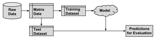
The procedure of partitioning data into training and test datasets that we used in previous chapters is known as the holdout method. As shown in the following diagram, the training dataset is used to generate the model, which is then applied to the test dataset to generate predictions for evaluation. Typically, about one-third of the data is held out for testing and two-thirds used for training, but this proportion can vary depending on the amount of data available. To ensure that the training and test data do not have systematic differences, examples are randomly divided into the two groups.

For the holdout method to result in a truly accurate estimate of future performance, at no time should results from the test dataset be allowed to influence the model. It is easy to unknowingly violate this rule by choosing a best model based upon the results of repeated testing. Instead, it is better to divide the original data so that in addition to the training and test datasets, a third validation dataset is available. The validation dataset would be used for iterating and refining the model or models chosen, leaving the test dataset to be used only once as a final step to report an estimated error rate for future predictions. A typical split between training, test, and validation would be 50 percent, 25 percent, and 25 percent respectively.

A simple method for creating holdout samples uses random number generators to assign records to partitions. This technique was first used in Chapter 5, Divide and Conquer – Classification Using Decision Trees and Rules to create training and test datasets.

Suppose we have a data frame named credit with 1000 rows of data. We can divide this into three partitions:

> random_ids <- order(runif(1000))
> credit_train <- credit[random_ids[1:500],]
> credit_validate <- credit[random_ids[501:750], ]
> credit_test <- credit[random_ids[751:1000], ]

The first line creates a vector of randomly ordered row IDs from 1 to 1000. These IDs are then used to divide the credit data frame into 500, 250, and 250 records comprising the training, validation, and test datasets.

One problem with holdout sampling is that each partition may have a larger or smaller proportion of some classes. In certain cases, particularly those in which a class is a very small proportion of the dataset, this can lead a class to be omitted from the training dataset—a significant problem, because the model cannot then learn this class.

In order to reduce the chance that this will occur, a technique called stratified random sampling can be used. Although, on average, a random sample will contain roughly the same proportion of class values as the full dataset, stratified random sampling ensures that the generated random partitions have approximately the same proportion of each class as the full dataset.

The caret package provides a createDataPartition() function that will create partitions based on stratified holdout sampling. Code for creating a stratified sample of training and test data for the credit dataset is shown in the following commands. To use the function, a vector of class values must be specified (here, default refers to whether a loan went into default), in addition to a parameter p, which specifies the proportion of instances to be included in the partition. The list = FALSE parameter prevents the result from being stored in list format:

> in_train <- createDataPartition(credit$default, p = 0.75,
    list = FALSE)
> credit_train <- credit[in_train, ]
> credit_test <- credit[-in_train, ]

The in_train vector indicates row numbers included in the training sample. We can use these row numbers to select examples for the credit_train data frame. Similarly, by using a negative symbol, we can use the rows not found in the in_train vector for the credit_test dataset.

Although it distributes the classes evenly, stratified sampling does not guarantee other types of representativeness. Some samples may have too many or too few difficult cases, easy-to-predict cases, or outliers. This is especially true for smaller datasets, which may not have a large enough portion of such cases to divide among training and test sets.

In addition to potentially biased samples, another problem with the holdout method is that substantial portions of data must be reserved for testing and validating the model. Since these data cannot be used to train the model until its performance has been measured, the performance estimates are likely to be overly conservative.

A technique called repeated holdout is sometimes used to mitigate the problems of randomly composed training datasets. The repeated holdout method is a special case of the holdout method that uses the average result from several random holdout samples to evaluate a model's performance. As multiple holdout samples are used, it is less likely that the model is trained or tested on non-representative data. We'll expand on this idea in the next section.

The repeated holdout is the basis of a technique known as k-fold cross-validation (or k-fold CV), which has become the industry standard for estimating model performance. But rather than taking repeated random samples that could potentially use the same record more than once, k-fold CV randomly divides the data into k completely separate random partitions called folds.

Although k can be set to any number, by far the most common convention is to use 10-fold cross-validation (10-fold CV). Why 10 folds? Empirical evidence suggests that there is little added benefit to using a greater number. For each of the 10 folds (each comprising 10 percent of the total data), a machine learning model is built on the remaining 90 percent of data. The fold's matching 10 percent sample is then used for model evaluation. After the process of training and evaluating the model has occurred for 10 times (with 10 different training/testing combinations), the average performance across all folds is reported.

Datasets for cross-validation can be created using the createFolds() function in the caret package. Similar to the stratified random holdout sampling, this function will attempt to maintain the same class balance in each of the folds as in the original dataset. The following is the command for creating 10 folds:

> folds <- createFolds(credit$default, k = 10)

The result of the createFolds() function is a list of vectors storing the row numbers for each of the k = 10 requested folds. We can peek at the contents using str():

> str(folds)
List of 10
 $ Fold01: int [1:100] 1 5 12 13 19 21 25 32 36 38 ...
 $ Fold02: int [1:100] 16 49 78 81 84 93 105 108 128 134 ...
 $ Fold03: int [1:100] 15 48 60 67 76 91 102 109 117 123 ...
 $ Fold04: int [1:100] 24 28 59 64 75 85 95 97 99 104 ...
 $ Fold05: int [1:100] 9 10 23 27 29 34 37 39 53 61 ...
 $ Fold06: int [1:100] 4 8 41 55 58 103 118 121 144 146 ...
 $ Fold07: int [1:100] 2 3 7 11 14 33 40 45 51 57 ...
 $ Fold08: int [1:100] 17 30 35 52 70 107 113 129 133 137 ...
 $ Fold09: int [1:100] 6 20 26 31 42 44 46 63 79 101 ...
 $ Fold10: int [1:100] 18 22 43 50 68 77 80 88 106 111 ...

Here, we see that the first fold is named Fold01, and stores 100 integers indicating the 100 rows in the credit data frame for the first fold. To create training and test datasets to build and evaluate a model, one more step is needed. The following commands show how to create data for the first fold. Just as we had done with stratified holdout sampling, we'll assign the selected examples to the training dataset and use the negative symbol to assign everything else to the test dataset:

> credit01_train <- credit[folds$Fold01, ]
> credit01_test <- credit[-folds$Fold01, ]

To perform the full 10-fold CV, this step would need to be repeated a total of 10 times, building a model, and then calculating the model's performance each time. At the end, the performance measures would be averaged to obtain the overall performance. Thankfully, we can automate this task by applying several of the techniques we've learned before.

To demonstrate the process, we'll estimate the kappa statistic for a C5.0 decision tree model of the credit data using 10-fold CV. First, we need to load caret (for creating the folds), C50 (for the decision tree), and irr (for calculating kappa). The latter two packages were chosen for illustrative purposes; if you desire, you can use a different model or a different performance measure with the same series of steps.

> library(caret)
> library(C50)
> library(irr)

Next, we'll create a list of 10 folds as we have done previously. The set.seed() function is used here to ensure that the results are consistent if you run the same code again:

> set.seed(123)
> folds <- createFolds(credit$default, k = 10)

Finally, we will apply a series of identical steps to the list of folds using the lapply() function. As shown in the following code, because there is no existing function that does exactly what we need, we must define our own function to pass to lapply(). Our custom function divides the credit data frame into training and test data, creates a decision tree using the C5.0() function on the training data, generates a set of predictions from the test data, and compares the predicted and actual values using the kappa2() function:

> cv_results <- lapply(folds, function(x) {
    credit_train <- credit[x, ]
    credit_test <- credit[-x, ]
    credit_model <- C5.0(default ~ ., data = credit_train)
    credit_pred <- predict(credit_model, credit_test)
    credit_actual <- credit_test$default
    kappa <- kappa2(data.frame(credit_actual, credit_pred))$value
    return(kappa)
  })

The resulting kappa statistics are compiled into a list stored in the cv_results object, which we can examine using str():

> str(cv_results)
List of 10
 $ Fold01: num 0.283
 $ Fold02: num 0.108
 $ Fold03: num 0.326
 $ Fold04: num 0.162
 $ Fold05: num 0.243
 $ Fold06: num 0.257
 $ Fold07: num 0.0355
 $ Fold08: num 0.0761
 $ Fold09: num 0.241
 $ Fold10: num 0.253

In this way, we've transformed our list of IDs for 10 folds into a list of kappa statistics. There's just one more step remaining: we need to calculate the average of these 10 values. Although you will be tempted to type mean(cv_results), because cv_results is not a numeric vector the result would be an error. Instead, use the unlist() function, which eliminates the list structure and reduces cv_results to a numeric vector. From there, we can calculate the mean kappa as expected:

> mean(unlist(cv_results))
[1] 0.1984929

Unfortunately, this kappa statistic is fairly low—in fact, this corresponds to "poor" on the interpretation scale—which suggests that the credit scoring model does not perform much better than random chance. In the next chapter, we'll examine automated methods based on 10-fold CV that can assist us with improving the performance of this model.

A slightly less popular, but still fairly widely-used alternative to k-fold CV is known as bootstrap sampling, the bootstrap, or bootstrapping for short. Generally speaking, these refer to statistical methods of using random samples of data to estimate properties of a larger set. When this principle is applied to machine learning model performance, it implies the creation of several randomly-selected training and test datasets, which are then used to estimate performance statistics. The results from the various random datasets are then averaged to obtain a final estimate of future performance.

So, what makes this procedure different from k-fold CV? Where cross-validation divides the data into separate partitions, in which each example can appear only once, the bootstrap allows examples to be selected multiple times through a process of sampling with replacement. This means that from the original dataset of n examples, the bootstrap procedure will create one or more new training datasets that also contain n examples, some of which are repeated. The corresponding test datasets are then constructed from the set of examples that were not selected for the respective training datasets.

Using sampling with replacement as described previously, the probability that any given instance is included in the training dataset is 63.2 percent. Consequently, the probability of any instance being in the test dataset is 36.8 percent. In other words, the training data represents only 63.2 percent of available examples, some of which are repeated. In contrast with 10-fold CV, which uses 90 percent of examples for training, the bootstrap sample is less representative of the full dataset.

As a model trained on only 63.2 percent of the training data is likely to perform worse than a model trained on a larger training set, the bootstrap's performance estimates may be substantially lower than what will be obtained when the model is later trained on the full dataset. A special case of bootstrapping known as the 0.632 bootstrap accounts for this by calculating the final performance measure as a function of performance on both the training data (which is overly optimistic) and the test data (which is overly pessimistic). The final error rate is then estimated as:

One advantage of the bootstrap over cross-validation is that it tends to work better with very small datasets. Additionally, bootstrap sampling has applications beyond performance measurement. In particular, in the following chapter we'll learn how the principles of bootstrap sampling can be used to improve model performance.