When a sports team falls short of meeting its goal—whether it is to obtain an Olympic gold medal, a league championship, or a world record time—it must begin a process of searching for improvements to avoid a similar fate in the future. Imagine that you're the coach of such a team. How would you spend your practice sessions? Perhaps you'd direct the athletes to train harder or train differently in order to maximize every bit of their potential. Or, you might place a greater emphasis on teamwork, which could utilize the athletes' strengths and weaknesses more smartly.
Now imagine that you're the coach tasked with finding a world champion machine learning algorithm—perhaps to enter a competition, such as those posted on the Kaggle website (http://www.kaggle.com/competitions), to win the million dollar Netflix Prize (http://www.netflixprize.com/), or simply to improve the bottom line for your business. Where do you begin?
Although the context of the competition may differ, many strategies one might use to improve a sports team's performance can also be used to improve the performance of statistical learners. As the coach, it is your job to find the combination of training techniques and teamwork skills that allow you to meet your performance goals.
This chapter builds upon the material covered in this book so far to introduce a set of techniques for improving the predictive performance of machine learners. You will learn:
- How to fine-tune the performance of machine learning models by searching for the optimal set of training conditions
- Methods for combining models into groups that use teamwork to tackle the most challenging problems
- Cutting edge techniques for getting the maximum level of performance out of machine learners
Not all of these methods will be successful on every problem. Yet if you look at the winning entries to machine learning competitions, you're likely to find at least one of them has been employed. To remain competitive, you too will need to add these skills to your repertoire.
Some learning problems are well suited to the stock models presented in previous chapters. In such cases, you may not need to spend much time iterating and refining the model; it may perform well enough as it is. On the other hand, some problems are inherently more difficult. The underlying concepts to be learned may be extremely complex, requiring an understanding of many subtle relationships, or it may have elements of random chance, making it difficult to define the signal within the noise.
Developing models that perform extremely well on such difficult problems is every bit an art as it is a science. Sometimes, a bit of intuition is helpful when trying to identify areas where performance can be improved. In other cases, finding improvements will require a brute-force, trial and error approach. Of course, the process of searching numerous possible improvements can be aided by the use of automated programs.
In Chapter 5, Divide and Conquer – Classification Using Decision Trees and Rules, we attempted a difficult problem: identifying loans that were likely to enter into default. Although we were able to use performance tuning methods to obtain a respectable classification accuracy of about 72 percent, upon a more careful examination in Chapter 10, Evaluating Model Performance, we realized that the high accuracy was a bit misleading. In spite of the reasonable accuracy, the kappa statistic was only about 0.20, which suggested that the model was actually performing somewhat poorly. In this section, we'll revisit the credit scoring model to see if we can improve the results.
You will recall that we first used a stock C5.0 decision tree to build the classifier for the credit data. We then attempted to improve its performance by adjusting the trials parameter to increase the number of boosting iterations. By increasing the trials from the default of 1 up to the values of 10 and 100, we were able to increase the model's accuracy. This process of adjusting the model fit options is called
parameter tuning.
Parameter tuning is not limited to decision trees. For instance, we tuned k-nearest neighbor models when we searched for the best value of k, and used a number of options for neural networks and support vector machines, such as adjusting the number of nodes, hidden layers, or choosing different kernel functions. Most machine learning algorithms allow you to adjust at least one parameter, and the most sophisticated models offer a large number of ways to tweak the model fit to your liking. Although this allows the model to be tailored closely to the data, the complexity of all the possible options can be daunting. A more systematic approach is warranted.
Rather than choosing arbitrary values for each of the model's parameters—a task that is not only tedious but somewhat unscientific—it is better to conduct a search through many possible parameter values to find the best combination.
The
caret package, which we used extensively in Chapter 10, Evaluating Model Performance, provides tools to assist with automated parameter tuning. The core functionality is provided by a train() function that serves as a standardized interface to train 150 different machine learning models for both classification and regression tasks. By using this function, it is possible to automate the search for optimal models using a choice of evaluation methods and metrics.
Automated parameter tuning requires you to consider three questions:
- What type of machine learning model (and/or specific implementation of the algorithm) should be trained on the data?
- Which model parameters can be adjusted, and how extensively should they be tuned to find the optimal settings?
- What criteria should be used to evaluate the models to find the best candidate?
To answer the first question involves finding a well-suited match between the machine learning task and one of the 150 models. Obviously, this requires an understanding of the breadth and depth of machine learning models. This book provides the background needed for the former, while additional practice will help with the latter. Additionally, it can help to work through a process of elimination: nearly half of the models can be eliminated depending on whether the task is classification or regression; others can be excluded based on the format of the data or the need to avoid black box models, and so on. In any case, there's also no reason you can't try several approaches and compare the best result of each.
Addressing the second question is a matter largely dictated by the choice of model, since each algorithm utilizes a unique set of parameters. The available tuning parameters for each of the predictive models covered in this book are listed in the following table. Keep in mind that although some models have additional options not shown, only those listed in the table are supported by caret for automatic tuning.
Note
For a complete list of the 150 models and corresponding tuning parameters covered by caret, refer to the table provided by package author Max Kuhn at: http://caret.r-forge.r-project.org/modelList.html
|
Model |
Learning task |
Method name |
Parameters |
|---|---|---|---|
|
k-Nearest Neighbors |
Classification |
|
|
|
Naïve Bayes |
Classification |
|
|
|
Decision Trees |
Classification |
|
|
|
OneR Rule Learner |
Classification |
|
None |
|
RIPPER Rule Learner |
Classification |
|
|
|
Linear Regression |
Regression |
|
None |
|
Regression Trees |
Regression |
|
|
|
Model Trees |
Regression |
|
|
|
Neural Networks |
Dual use |
|
|
|
Support Vector Machines (Linear Kernel) |
Dual use |
|
|
|
Support Vector Machines (Radial Basis Kernel) |
Dual use |
|
|
|
Random Forests |
Dual use |
|
|
The goal of automatic tuning is to search a set of candidate models comprising a matrix, or grid, of possible combinations of parameters. Because it is impractical to search every conceivable parameter value, only a subset of possibilities is used to construct the grid. By default, caret searches at most three values for each of p parameters, which means that 3^p candidate models will be tested. For example, by default, the automatic tuning of k-nearest neighbors will compare 3^1 = 3 candidate models, for instance, one each of k=5, k=7, and k=9. Similarly, tuning a decision tree could result in a comparison of up to 27 different candidate models, comprising the grid of 3^3 = 27 possible combinations of model, trials, and winnow settings. In practice, however, only 12 models are actually tested. This is because the model and winnow parameters can only take two values (tree versus rules and TRUE versus FALSE, respectively), which makes the grid size 3*2*2 = 12.
The third and final step in automatic model tuning involves choosing an approach to identify the best model among the candidates. This uses the methods discussed in Chapter 10, Evaluating Model Performance such as the choice of resampling strategy to create training and test datasets, and the use of model performance statistics to measure the predictive accuracy.
All of the resampling strategies and many of the performance statistics we've learned are supported by caret. These include statistics such as accuracy and kappa (for classifiers) and R-squared or RMSE (for numeric models). Cost-sensitive measures like sensitivity, specificity, and area under the ROC curve (AUC) can also be used if desired.
By default, when choosing the best model, caret will select the model with the largest value of the desired performance measure. Because this practice sometimes results in the selection of models that achieve marginal performance improvements via large increases in model complexity, alternative model selection functions are provided.
Given the wide variety of options, it is helpful that many of the defaults are reasonable. For instance, it will use prediction accuracy on a bootstrap sample to choose the best performer for classification models. Beginning with these default values, we can then tweak the train() function to design a wide variety of experiments.
To illustrate the process of tuning a model, let's begin by observing what happens when we attempt to tune the credit scoring model using the caret package's default settings. From there, we will learn how adjust the options to our liking.
The simplest way to tune a learner requires only that you specify a model type via the method parameter. Since we used C5.0 decision trees previously with the credit model, we'll continue our work by optimizing this learner. The basic train() command for tuning a C5.0 decision tree using the default settings is as follows:
> library(caret)
> set.seed(300)
> m <- train(default ~ ., data = credit, method = "C5.0")
First, the set.seed() function is used to initialize R's random number generator to a set starting position. You may recall that we have used this function in several prior chapters. By setting the seed parameter (in this case to the arbitrary number 300), the random numbers will follow a predefined sequence. This allows simulations like train(), which use random sampling, to be repeated with identical results—a very helpful feature if you are sharing code or attempting to replicate a prior result.
Next, the R formula interface is used to define a tree as default ~ .. This models loan default status (yes or no) using all of the other features in the credit data frame. The parameter method = "C5.0" tells caret to use the C5.0 decision tree algorithm.
After you've entered the preceding command, there may be a significant delay (dependent upon your computer's capabilities) as the tuning process occurs. Even though this is a fairly small dataset, a substantial amount of calculation must occur. R is repeatedly generating random samples of data, building decision trees, computing performance statistics, and evaluating the result.
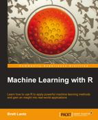
The result of the experiment is saved in an object, which we named m. If you would like a peek at the object's contents, the command str(m) will list all the associated data—but this can be quite overwhelming. Instead, simply type the name of the object for a condensed summary of the results. For instance, typing m yields the following output:
The summary includes four main components:
- A brief description of the input dataset: If you are familiar with your data and have applied the
train()function correctly, none of this information should come as a surprise. - A report of preprocessing and resampling methods applied: Here we see that 25 bootstrap samples, each including 1000 examples, were used to train the models.
- A list of candidate models evaluated: In this section, we can confirm that 12 different models were tested, based on combinations of three C5.0 tuning parameters:
model,trials, andwinnow. The average and standard deviation (labeledSD) of the accuracy and kappa statistics for each candidate model are also shown. - The choice of best model: As noted, the model with the largest accuracy value (
0.73) was chosen as the best. This was the model that used amodel = tree,trials = 20, andwinnow = FALSE.
The train() function uses the tuning parameters from the best model (as indicated by #4 previously) to build a model on the full input dataset, which is stored in the m object as m$finalModel. In most cases, you will not need to work directly with the finalModel sub-object. Instead, using the predict() function with the m object will generate predictions as expected, while also providing added functionality that will be described shortly. For example, to apply the best model to make predictions on the training data, you would use the following commands:
> p <- predict(m, credit)
The resulting vector of predictions works just as we have done many times before:
> table(p, credit$default)

p      no yes
  no  700   2
  yes   0 298
Of the 1000 examples used for training the final model, only two were misclassified. Keep in mind that this is the resubstitution error and should not be viewed as indicative of performance on unseen data. The bootstrap estimate of 73 percent (shown in the summary output) is a more realistic estimate of future performance.
As mentioned previously, there are additional benefits of using predict(), directly on train() objects rather than using the stored finalModel directly or training a new model using the optimized parameters.
First, any data preprocessing steps that the train() function applied to the data will be similarly applied to the data used for generating predictions. This includes transformations like centering and scaling (that is, when using k-nearest neighbors), missing value imputation, and others. This ensures that the data preparation steps used for developing the model remain in place when the model is deployed.
Second, the predict() function for caret models provides a standardized interface for obtaining predicted class values and predicted class probabilities—even for models that ordinarily would require additional steps to obtain this information. The predicted classes are provided by default as follows:
> head(predict(m, credit))
[1] no  yes no  no  yes no
Levels: no yes
To obtain the estimated probabilities for each class, add an additional parameter specifying type = "prob":
> head(predict(m, credit, type = "prob"))
         no        yes
1 0.9606970 0.03930299
2 0.1388444 0.86115561
3 1.0000000 0.00000000
4 0.7720279 0.22797208
5 0.2948062 0.70519385
6 0.8583715 0.14162851
Even in cases where the underlying model refers to the prediction probabilities using a different string (for example, "raw" for a naiveBayes model), caret automatically translates type = "prob" to the appropriate string behind the scenes.
The decision tree we created previously demonstrates the caret package's ability to produce an optimized model with minimal intervention. The default settings allow strongly performing models to be created easily. However, without digging deeper, you may miss out on the upper echelon of performance. Or perhaps you want to change the default evaluation criteria to something more appropriate for your learning problem. Each step in the process can be customized to your learning task.
To illustrate this flexibility, let's modify our work on the credit decision tree explained previously to mirror the process we had used in Chapter 10, Evaluating Model Performance. If you recall from that chapter, we had estimated the kappa statistic using 10-fold cross-validation. We'll do the same here, using kappa to optimize the boosting parameter of the decision tree (boosting the accuracy of decision trees was previously covered in Chapter 5, Divide and Conquer – Classification Using Decision Trees and Rules).
The trainControl() function is used to create a set of configuration options known as a control object, which can be used with the train() function. These options allow for the management of model evaluation criteria such as the resampling strategy and the measure used for choosing the best model. Although this function can be used to modify nearly every aspect of a tuning experiment, we'll focus on two important parameters: method and selectionFunction.
For the trainControl() function, the method parameter is used to set the resampling method, such as holdout sampling or k-fold cross-validation. The following table lists the shortened name string caret uses to call the method, as well as any additional parameters for adjusting the sample size and number of iterations. Although the default options for these resampling methods follow popular convention, you may choose to adjust these depending upon the size of your dataset and the complexity of your model.
|
Resampling method |
Method name |
Additional options and default values |
|---|---|---|
|
Holdout sampling |
|
|
|
k-fold cross-validation |
|
|
|
Repeated k-fold cross-validation |
|
|
|
Bootstrap sampling |
|
|
|
0.632 bootstrap |
|
|
|
Leave-one-out cross-validation |
|
None |
The trainControl() parameter selectionFunction can be used to choose a function that selects the optimal model among the various candidates. Three such functions are included. The best function simply chooses the candidate with the best value on the specified performance measure. This is used by default. The other two functions are used to choose the most parsimonious (that is, simplest) model that is within a certain threshold of the best model's performance. The oneSE function chooses the simplest candidate within one standard error of the best performance, and tolerance uses the simplest candidate within a user-specified percentage.
To create a control object named ctrl that uses 10-fold cross-validation and the oneSE selection function, use the following command. Note that number = 10 is included only for clarity; since this is the default value for method = "cv", it could have been omitted.
> ctrl <- trainControl(method = "cv", number = 10,
                       selectionFunction = "oneSE")
We'll use the result of this function shortly.
In the meantime, the next step in defining our experiment is to create a grid of parameters to optimize. The grid must include a column for each parameter in the desired model, prefixed by a period. Since we are using a C5.0 decision tree, this means we'll need columns with the names .model, .trials, and .winnow. For other models, refer to the table presented earlier in this chapter. Each row in the data frame represents a particular combination of parameter values.
Rather than creating this data frame ourselves—a difficult task if there are many possible combinations of parameter values—we can use the expand.grid() function, which creates data frames from the combinations of all values supplied. For example, suppose we would like to hold constant model = "tree" and winnow = "FALSE" while searching eight different values of trials. This can be created as:
> grid <- expand.grid(.model = "tree",
                      .trials = c(1, 5, 10, 15, 20, 25, 30, 35),
                      .winnow = "FALSE")
The resulting grid data frame contains 1*8*1 = 8 rows:
> grid
  .model .trials .winnow
1   tree       1   FALSE
2   tree       5   FALSE
3   tree      10   FALSE
4   tree      15   FALSE
5   tree      20   FALSE
6   tree      25   FALSE
7   tree      30   FALSE
8   tree      35   FALSE
Each row will be used to generate a candidate model for evaluation, built using that row's combination of model parameters.
Given this search grid and the control list created previously, we are ready to run a thoroughly customized train() experiment. As before, we'll set the random seed to ensure repeatable results. But this time, we'll pass our control object and tuning grid while adding a parameter metric = "Kappa", indicating the statistic to be used by the model evaluation function—in this case, "oneSE". The full command is as follows:
> set.seed(300)
> m <- train(default ~ ., data = credit, method = "C5.0",
             metric = "Kappa",
             trControl = ctrl,
             tuneGrid = grid)
This results in an object that we can view as before:
> m
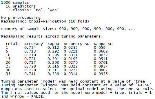
Although much of the output is similar to the previously tuned model, there are a few differences of note. Because 10-fold cross-validation was used, the sample size to build each candidate model was reduced to 900 rather than the 1000 used in the bootstrap. As we requested, eight candidate models were tested. Additionally, because model and winnow were held constant, their values are no longer shown in the results; instead, they are listed as a footnote.
The best model here differs quite significantly from the prior trial. Before, the best model used trials = 20 whereas here, the best used trials = 1. This seemingly odd finding is due to the fact that we used the oneSE rule rather the best rule to select the optimal model. Even though the 35-trial model offers the best raw performance according to kappa, the 1-trial model offers nearly the same performance yet is a much simpler model. Not only are simple models more computationally efficient, simple models are preferable because they reduce the chance of overfitting the training data.