Both PCA and LDA are linear transformation techniques that can be used to reduce the number of dimensions in a dataset; the former is an unsupervised algorithm, whereas the latter is supervised. Thus, we might intuitively think that LDA is a superior feature extraction technique for classification tasks compared to PCA. However, A.M. Martinez reported that preprocessing via PCA tends to result in better classification results in an image recognition task in certain cases, for instance if each class consists of only a small number of samples (PCA Versus LDA, A. M. Martinez and A. C. Kak, IEEE Transactions on Pattern Analysis and Machine Intelligence, 23(2): 228-233, 2001).

The following figure summarizes the concept of LDA for a two-class problem. Samples from class 1 are shown as circles, and samples from class 2 are shown as crosses:

A linear discriminant, as shown on the x-axis (LD 1), would separate the two normal distributed classes well. Although the exemplary linear discriminant shown on the y-axis (LD 2) captures a lot of the variance in the dataset, it would fail as a good linear discriminant since it does not capture any of the class-discriminatory information.

One assumption in LDA is that the data is normally distributed. Also, we assume that the classes have identical covariance matrices and that the samples are statistically independent of each other. However, even if one or more of those assumptions are (slightly) violated, LDA for dimensionality reduction can still work reasonably well (Pattern Classification 2nd Edition, R. O. Duda, P. E. Hart, and D. G. Stork, New York, 2001).

Before we dive into the code implementation, let's briefly summarize the main steps that are required to perform LDA:

As we can see, LDA is quite similar to PCA in the sense that we are decomposing matrices into eigenvalues and eigenvectors, which will form the new lower-dimensional feature space. However, as mentioned before, LDA takes class label information into account, which is represented in the form of the mean vectors computed in step 2. In the following sections, we will discuss these seven steps in more detail, accompanied by illustrative code implementations.

Since we already standardized the features of the Wine dataset in the PCA section at the beginning of this chapter, we can skip the first step and proceed with the calculation of the mean vectors, which we will use to construct the within-class scatter matrix and between-class scatter matrix, respectively. Each mean vector stores the mean feature value with respect to the samples of class i:

This results in three mean vectors:

>>> np.set_printoptions(precision=4)
>>> mean_vecs = []
>>> for label in range(1,4):
...     mean_vecs.append(np.mean(
...                X_train_std[y_train==label], axis=0))
...     print('MV %s: %s
' %(label, mean_vecs[label-1]))
MV 1: [ 0.9066 -0.3497  0.3201 -0.7189  0.5056  0.8807  0.9589 -0.5516  0.5416  0.2338  0.5897  0.6563  1.2075]

MV 2: [-0.8749 -0.2848 -0.3735  0.3157 -0.3848 -0.0433  0.0635 -0.0946  0.0703 -0.8286  0.3144  0.3608 -0.7253]

MV 3: [ 0.1992  0.866   0.1682  0.4148 -0.0451 -1.0286 -1.2876  0.8287 -0.7795  0.9649 -1.209  -1.3622 -0.4013]

Using the mean vectors, we can now compute the within-class scatter matrix :

This is calculated by summing up the individual scatter matrices of each individual class i:

>>> d = 13 # number of features
>>> S_W = np.zeros((d, d))
>>> for label, mv in zip(range(1, 4), mean_vecs):
...     class_scatter = np.zeros((d, d))
>>>     for row in X_train_std[y_train == label]:
...         row, mv = row.reshape(d, 1), mv.reshape(d, 1)  
...         class_scatter += (row - mv).dot((row - mv).T)
...     S_W += class_scatter
>>> print('Within-class scatter matrix: %sx%s' % (
...       S_W.shape[0], S_W.shape[1]))
Within-class scatter matrix: 13x13

The assumption that we are making when we are computing the scatter matrices is that the class labels in the training set are uniformly distributed. However, if we print the number of class labels, we see that this assumption is violated:

>>> print('Class label distribution: %s' 
...       % np.bincount(y_train)[1:])
Class label distribution: [41 50 33]

Thus, we want to scale the individual scatter matrices before we sum them up as scatter matrix . When we divide the scatter matrices by the number of class-samples , we can see that computing the scatter matrix is in fact the same as computing the covariance matrix —the covariance matrix is a normalized version of the scatter matrix:

>>> d = 13 # number of features
>>> S_W = np.zeros((d, d))
>>> for label,mv in zip(range(1, 4), mean_vecs):
...     class_scatter = np.cov(X_train_std[y_train==label].T)
...     S_W += class_scatter
>>> print('Scaled within-class scatter matrix: %sx%s' 
...       % (S_W.shape[0], S_W.shape[1]))
Scaled within-class scatter matrix: 13x13

After we computed the scaled within-class scatter matrix (or covariance matrix), we can move on to the next step and compute the between-class scatter matrix :

Here, is the overall mean that is computed, including samples from all classes:

>>> mean_overall = np.mean(X_train_std, axis=0)
>>> d = 13  # number of features
>>> S_B = np.zeros((d, d))
>>> for i, mean_vec in enumerate(mean_vecs):
...     n = X_train[y_train == i + 1, :].shape[0]
...     mean_vec = mean_vec.reshape(d, 1)  # make column vector
...     mean_overall = mean_overall.reshape(d, 1) 
...     S_B += n * (mean_vec - mean_overall).dot(
...                (mean_vec - mean_overall).T)
>>> print('Between-class scatter matrix: %sx%s' % (
...                S_B.shape[0], S_B.shape[1]))
			Between-class scatter matrix: 13x1

The remaining steps of the LDA are similar to the steps of the PCA. However, instead of performing the eigendecomposition on the covariance matrix, we solve the generalized eigenvalue problem of the matrix :

>>> eigen_vals, eigen_vecs =
...            np.linalg.eig(np.linalg.inv(S_W).dot(S_B))

After we computed the eigenpairs, we can now sort the eigenvalues in descending order:

>>> eigen_pairs = [(np.abs(eigen_vals[i]), eigen_vecs[:,i]) 
...              for i in range(len(eigen_vals))]
>>> eigen_pairs = sorted(eigen_pairs, 
...               key=lambda k: k[0], reverse=True)
>>> print('Eigenvalues in descending order:
')
>>> for eigen_val in eigen_pairs:
...     print(eigen_val[0])


Eigenvalues in descending order:

349.617808906
172.76152219
3.78531345125e-14
2.11739844822e-14
1.51646188942e-14
1.51646188942e-14
1.35795671405e-14
1.35795671405e-14
7.58776037165e-15
5.90603998447e-15
5.90603998447e-15
2.25644197857e-15
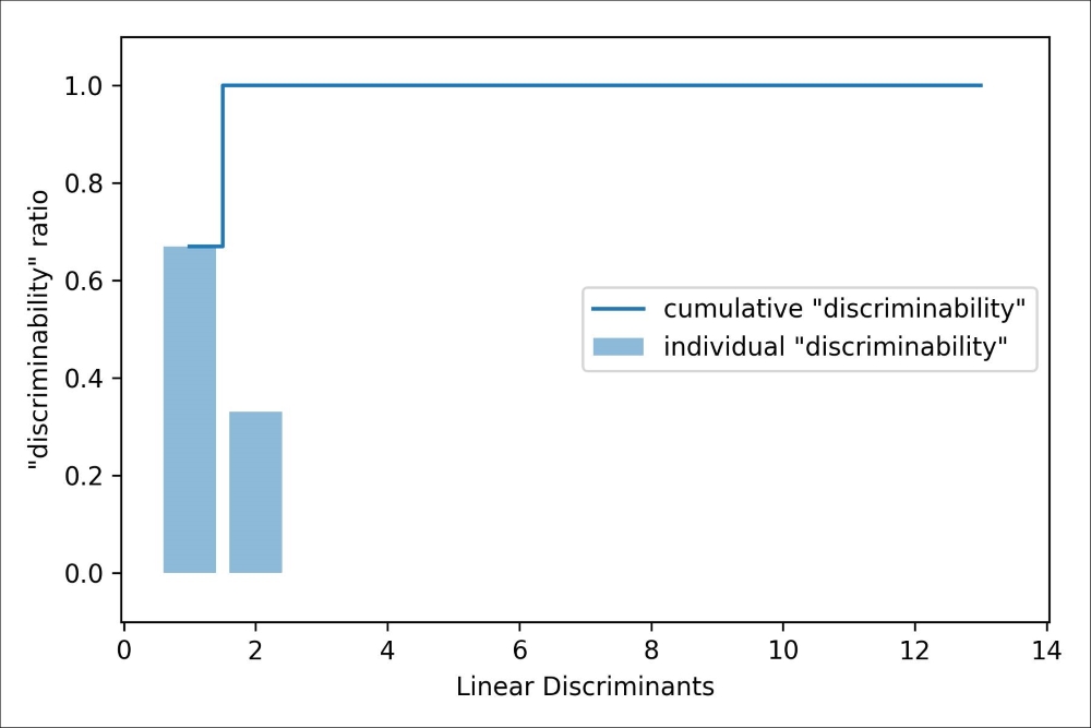
0.0

In LDA, the number of linear discriminants is at most c−1, where c is the number of class labels, since the in-between scatter matrix is the sum of c matrices with rank 1 or less. We can indeed see that we only have two nonzero eigenvalues (the eigenvalues 3-13 are not exactly zero, but this is due to the floating point arithmetic in NumPy).

To measure how much of the class-discriminatory information is captured by the linear discriminants (eigenvectors), let's plot the linear discriminants by decreasing eigenvalues similar to the explained variance plot that we created in the PCA section. For simplicity, we will call the content of class-discriminatory information discriminability:

>>> tot = sum(eigen_vals.real)
>>> discr = [(i / tot) for i in sorted(eigen_vals.real, reverse=True)]
>>> cum_discr = np.cumsum(discr)
>>> plt.bar(range(1, 14), discr, alpha=0.5, align='center',
...         label='individual "discriminability"')
>>> plt.step(range(1, 14), cum_discr, where='mid',
...          label='cumulative "discriminability"')
>>> plt.ylabel('"discriminability" ratio')
>>> plt.xlabel('Linear Discriminants')
>>> plt.ylim([-0.1, 1.1])
>>> plt.legend(loc='best')
>>> plt.show()

As we can see in the resulting figure, the first two linear discriminants alone capture 100 percent of the useful information in the Wine training dataset:

Let's now stack the two most discriminative eigenvector columns to create the transformation matrix W:

>>> w = np.hstack((eigen_pairs[0][1][:, np.newaxis].real,
...                eigen_pairs[1][1][:, np.newaxis].real))
>>> print('Matrix W:
', w)
Matrix W:
 [[-0.1481 -0.4092]
 [ 0.0908 -0.1577]
 [-0.0168 -0.3537]
 [ 0.1484  0.3223]
 [-0.0163 -0.0817]
 [ 0.1913  0.0842]
 [-0.7338  0.2823]
 [-0.075  -0.0102]
 [ 0.0018  0.0907]
 [ 0.294  -0.2152]
 [-0.0328  0.2747]
 [-0.3547 -0.0124]
 [-0.3915 -0.5958]]

Using the transformation matrix W that we created in the previous subsection, we can now transform the training dataset by multiplying the matrices:

>>> X_train_lda = X_train_std.dot(w)
>>> colors = ['r', 'b', 'g']
>>> markers = ['s', 'x', 'o']
>>> for l, c, m in zip(np.unique(y_train), colors, markers):
...     plt.scatter(X_train_lda[y_train==l, 0], 
...                 X_train_lda[y_train==l, 1] * (-1), 
...                 c=c, label=l, marker=m)
>>> plt.xlabel('LD 1')
>>> plt.ylabel('LD 2')
>>> plt.legend(loc='lower right')
>>> plt.show()

As we can see in the resulting plot, the three wine classes are now perfectly linearly separable in the new feature subspace:

The step-by-step implementation was a good exercise to understand the inner workings of an LDA and understand the differences between LDA and PCA. Now, let's look at the LDA class implemented in scikit-learn:

>>> from sklearn.discriminant_analysis import 
...    LinearDiscriminantAnalysis as LDA
>>> lda = LDA(n_components=2)
>>> X_train_lda = lda.fit_transform(X_train_std, y_train)

Next, let's see how the logistic regression classifier handles the lower-dimensional training dataset after the LDA transformation:

>>> lr = LogisticRegression()
>>> lr = lr.fit(X_train_lda, y_train)
>>> plot_decision_regions(X_train_lda, y_train, classifier=lr)
>>> plt.xlabel('LD 1')
>>> plt.ylabel('LD 2')
>>> plt.legend(loc='lower left')
>>> plt.show()

Looking at the resulting plot, we see that the logistic regression model misclassifies one of the samples from class 2:

By lowering the regularization strength, we could probably shift the decision boundaries so that the logistic regression model classifies all samples in the training dataset correctly. However, and more importantly, let us take a look at the results on the test set:

>>> X_test_lda = lda.transform(X_test_std)
>>> plot_decision_regions(X_test_lda, y_test, classifier=lr)
>>> plt.xlabel('LD 1')
>>> plt.ylabel('LD 2')
>>> plt.legend(loc='lower left')
>>> plt.show()

As we can see in the following plot, the logistic regression classifier is able to get a perfect accuracy score for classifying the samples in the test dataset by only using a two-dimensional feature subspace instead of the original 13 Wine features: