In order to split the nodes at the most informative features, we need to define an objective function that we want to optimize via the tree learning algorithm. Here, our objective function is to maximize the information gain at each split, which we define as follows:

Here, f is the feature to perform the split, and are the dataset of the parent and jth child node, I is our impurity measure, is the total number of samples at the parent node, and is the number of samples in the jth child node. As we can see, the information gain is simply the difference between the impurity of the parent node and the sum of the child node impurities — the lower the impurity of the child nodes, the larger the information gain. However, for simplicity and to reduce the combinatorial search space, most libraries (including scikit-learn) implement binary decision trees. This means that each parent node is split into two child nodes, and :

Now, the three impurity measures or splitting criteria that are commonly used in binary decision trees are Gini impurity (), entropy (), and the classification error (). Let us start with the definition of entropy for all non-empty classes ():

Here, is the proportion of the samples that belong to class c for a particular node t. The entropy is therefore 0 if all samples at a node belong to the same class, and the entropy is maximal if we have a uniform class distribution. For example, in a binary class setting, the entropy is 0 if or . If the classes are distributed uniformly with and , the entropy is 1. Therefore, we can say that the entropy criterion attempts to maximize the mutual information in the tree.

Intuitively, the Gini impurity can be understood as a criterion to minimize the probability of misclassification:

Similar to entropy, the Gini impurity is maximal if the classes are perfectly mixed, for example, in a binary class setting ():

However, in practice both Gini impurity and entropy typically yield very similar results, and it is often not worth spending much time on evaluating trees using different impurity criteria rather than experimenting with different pruning cut-offs.

Another impurity measure is the classification error:

This is a useful criterion for pruning but not recommended for growing a decision tree, since it is less sensitive to changes in the class probabilities of the nodes. We can illustrate this by looking at the two possible splitting scenarios shown in the following figure:

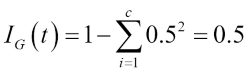
We start with a dataset at the parent node , which consists 40 samples from class 1 and 40 samples from class 2 that we split into two datasets, and . The information gain using the classification error as a splitting criterion would be the same () in both scenarios, A and B:

However, the Gini impurity would favor the split in scenario B () over scenario A (), which is indeed more pure:

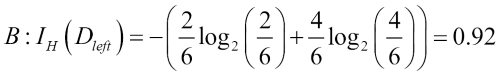
Similarly, the entropy criterion would also favor scenario B () over scenario A ():

For a more visual comparison of the three different impurity criteria that we discussed previously, let us plot the impurity indices for the probability range [0, 1] for class 1. Note that we will also add a scaled version of the entropy (entropy / 2) to observe that the Gini impurity is an intermediate measure between entropy and the classification error. The code is as follows:

>>> import matplotlib.pyplot as plt
>>> import numpy as np
>>> def gini(p):
...     return (p)*(1 - (p)) + (1 - p)*(1 - (1-p))
>>> def entropy(p):
...     return - p*np.log2(p) - (1 - p)*np.log2((1 - p))
>>> def error(p):
...     return 1 - np.max([p, 1 - p])
>>> x = np.arange(0.0, 1.0, 0.01)
>>> ent = [entropy(p) if p != 0 else None for p in x]
>>> sc_ent = [e*0.5 if e else None for e in ent]
>>> err = [error(i) for i in x]
>>> fig = plt.figure()
>>> ax = plt.subplot(111)
>>> for i, lab, ls, c, in zip([ent, sc_ent, gini(x), err], 
...                   ['Entropy', 'Entropy (scaled)', 
...                       'Gini Impurity', 
...                       'Misclassification Error'],
...                   ['-', '-', '--', '-.'],
...                   ['black', 'lightgray',
...                      'red', 'green', 'cyan']):
...     line = ax.plot(x, i, label=lab, 
...                    linestyle=ls, lw=2, color=c)
>>> ax.legend(loc='upper center', bbox_to_anchor=(0.5, 1.15),
...           ncol=5, fancybox=True, shadow=False)
>>> ax.axhline(y=0.5, linewidth=1, color='k', linestyle='--')
>>> ax.axhline(y=1.0, linewidth=1, color='k', linestyle='--')
>>> plt.ylim([0, 1.1])
>>> plt.xlabel('p(i=1)')
>>> plt.ylabel('Impurity Index')
>>> plt.show()

The plot produced by the preceding code example is as follows:

Decision trees can build complex decision boundaries by dividing the feature space into rectangles. However, we have to be careful since the deeper the decision tree, the more complex the decision boundary becomes, which can easily result in overfitting. Using scikit-learn, we will now train a decision tree with a maximum depth of 4, using Gini Impurity as a criterion for impurity. Although feature scaling may be desired for visualization purposes, note that feature scaling is not a requirement for decision tree algorithms. The code is as follows:

>>> from sklearn.tree import DecisionTreeClassifier
>>> tree = DecisionTreeClassifier(criterion='gini',
...                               max_depth=4, 
...                               random_state=1)
>>> tree.fit(X_train, y_train)
>>> X_combined = np.vstack((X_train, X_test))
>>> y_combined = np.hstack((y_train, y_test))
>>> plot_decision_regions(X_combined, 
...                       y_combined, 
...                       classifier=tree, 
...                       test_idx=range(105, 150))
>>> plt.xlabel('petal length [cm]')
>>> plt.ylabel('petal width [cm]')
>>> plt.legend(loc='upper left')
>>> plt.show()

After executing the code example, we get the typical axis-parallel decision boundaries of the decision tree:

A nice feature in scikit-learn is that it allows us to export the decision tree as a .dot file after training, which we can visualize using the GraphViz program, for example.

This program is freely available from http://www.graphviz.org and supported by Linux, Windows, and macOS. In addition to GraphViz, we will use a Python library called pydotplus, which has capabilities similar to GraphViz and allows us to convert .dot data files into a decision tree image file. After you installed GraphViz (by following the instructions on http://www.graphviz.org/Download.php), you can install pydotplus directly via the pip installer, for example, by executing the following command in your Terminal:

> pip3 install pydotplus

pip3 install graphviz
pip3 install pyparsing

The following code will create an image of our decision tree in PNG format in our local directory:

>>> from pydotplus import graph_from_dot_data
>>> from sklearn.tree import export_graphviz
>>> dot_data = export_graphviz(tree,
...                            filled=True, 
...                            rounded=True,
...                            class_names=['Setosa', 
...                                         'Versicolor',
...                                         'Virginica'],
...                            feature_names=['petal length', 
...                                           'petal width'],
...                            out_file=None) 
>>> graph = graph_from_dot_data(dot_data) 
>>> graph.write_png('tree.png')

By using the out_file=None setting, we directly assigned the dot data to a dot_data variable, instead of writing an intermediate tree.dot file to disk. The arguments for filled, rounded, class_names, and feature_names are optional but make the resulting image file visually more appealing by adding color, rounding the box edges, showing the name of the majority class label at each node, and displaying the feature names in the splitting criterion. These settings resulted in the following decision tree image:

Looking at the decision tree figure, we can now nicely trace back the splits that the decision tree determined from our training dataset. We started with 105 samples at the root and split them into two child nodes with 35 and 70 samples, using the petal width cut-off ≤ 0.75 cm. After the first split, we can see that the left child node is already pure and only contains samples from the Iris-setosa class (Gini Impurity = 0). The further splits on the right are then used to separate the samples from the Iris-versicolor and Iris-virginica class.

Looking at this tree, and the decision region plot of the tree, we see that the decision tree does a very good job of separating the flower classes. Unfortunately, scikit-learn currently does not implement functionality to manually post-prune a decision tree. However, we could go back to our previous code example, change the max_depth of our decision tree to 3, and compare it to our current model, but we leave this as an exercise for the interested reader.

Random forests have gained huge popularity in applications of machine learning during the last decade due to their good classification performance, scalability, and ease of use. Intuitively, a random forest can be considered as an ensemble of decision trees. The idea behind a random forest is to average multiple (deep) decision trees that individually suffer from high variance, to build a more robust model that has a better generalization performance and is less susceptible to overfitting. The random forest algorithm can be summarized in four simple steps:

We should note one slight modification in step 2 when we are training the individual decision trees: instead of evaluating all features to determine the best split at each node, we only consider a random subset of those.

Although random forests don't offer the same level of interpretability as decision trees, a big advantage of random forests is that we don't have to worry so much about choosing good hyperparameter values. We typically don't need to prune the random forest since the ensemble model is quite robust to noise from the individual decision trees. The only parameter that we really need to care about in practice is the number of trees k (step 3) that we choose for the random forest. Typically, the larger the number of trees, the better the performance of the random forest classifier at the expense of an increased computational cost.

Although it is less common in practice, other hyperparameters of the random forest classifier that can be optimized—using techniques we will discuss in Chapter 5, Compressing Data via Dimensionality Reduction—are the size n of the bootstrap sample (step 1) and the number of features d that is randomly chosen for each split (step 2.1), respectively. Via the sample size n of the bootstrap sample, we control the bias-variance tradeoff of the random forest.

Decreasing the size of the bootstrap sample increases the diversity among the individual trees, since the probability that a particular training sample is included in the bootstrap sample is lower. Thus, shrinking the size of the bootstrap samples may increase the randomness of the random forest, and it can help to reduce the effect of overfitting. However, smaller bootstrap samples typically result in a lower overall performance of the random forest, a small gap between training and test performance, but a low test performance overall. Conversely, increasing the size of the bootstrap sample may increase the degree of overfitting. Because the bootstrap samples, and consequently the individual decision trees, become more similar to each other, they learn to fit the original training dataset more closely.

In most implementations, including the RandomForestClassifier implementation in scikit-learn, the size of the bootstrap sample is chosen to be equal to the number of samples in the original training set, which usually provides a good bias-variance tradeoff. For the number of features d at each split, we want to choose a value that is smaller than the total number of features in the training set. A reasonable default that is used in scikit-learn and other implementations is , where m is the number of features in the training set.

Conveniently, we don't have to construct the random forest classifier from individual decision trees by ourselves because there is already an implementation in scikit-learn that we can use:

>>> from sklearn.ensemble import RandomForestClassifier
>>> forest = RandomForestClassifier(criterion='gini',
...                                 n_estimators=25,
...                                 random_state=1,
...                                 n_jobs=2)
>>> forest.fit(X_train, y_train)
>>> plot_decision_regions(X_combined, y_combined, 
...                classifier=forest, test_idx=range(105,150))
>>> plt.xlabel('petal length')
>>> plt.ylabel('petal width')
>>> plt.legend(loc='upper left')
>>> plt.show()

After executing the preceding code, we should see the decision regions formed by the ensemble of trees in the random forest, as shown in the following figure:

Using the preceding code, we trained a random forest from 25 decision trees via the n_estimators parameter and used the entropy criterion as an impurity measure to split the nodes. Although we are growing a very small random forest from a very small training dataset, we used the n_jobs parameter for demonstration purposes, which allows us to parallelize the model training using multiple cores of our computer (here two cores).