
CHAPTER 25
Technology Improvement: Application of Design of Experiments
The future belongs to those who believe in the beauty of their dreams
– Eleanor Roosevelt
SYNOPSIS
Design of experiments (DOE) is another important area of application of statistical methodology for planning, executing and analysis of experiments in such a way that it can address pre-determined questions on the effect of certain factors or combination of factors, called interaction on any response. One particular type of DOE called orthogonal array (OA), popularised by Dr. Taguchi, helps to design minimum number of experiments commensurate with the number and type of questions to be answered. A number of examples have been worked out to illustrate the use of OA design.
Statistics, a key technology
Professor P. C. Mahalanobis, the visionary Founder Director of Indian Statistical Institute, pioneered the concept of ‘Statistics, a key technology’ and promoted the extensive use of statistical technology in diverse areas of activity, notably national planning, economics, industry, science and technology. The characteristics that constitute the building blocks for establishing a culture of innovation and improvement practised and established by Prof. Mahalanobis at Indian Statistical Institute are the subject matter of Chapter 29.
Against this background, the present chapter gives a brief view on statistics and industrial experimentation and the uniqueness and ability of Taguchi’s methods (TM). If quality is to be built into products and processes then scientists, technologists, engineers and industrial researchers must be competent in using these valuable tools.
Industrial experimentation
Quality improvement has already been discussed. Significant and substantial improvement is achieved through derived changes in product design and process/technology upgradation. One of the efficient routes to achieve such improvements is through experimentation. Industrial enterprises are not new to experimentation. But what needs to gain ground is increased adoption of statistical approach to industrial experimentation and statistical methods of design of experiments (DOE). These help to ensure the following.
- Selection of experimental design based on statistical technology to find answers to specific questions of interest/value which can be formulated even beforehand.
- Meeting these requirements with the least number of experiments.
There are a number of excellent books on statistical design and analysis of industrial experiments which discuss various types of experimental designs and their corresponding methods of analysis that fit into a variety of industrial situations. Comparison between conventional and statistical methods of experimentation is summarised in Annexure 25A.
Taguchi’s methods
Dr. Genichi Taguchi, recipient of the prestigious Deming Prize in 1960, and Shewart Model in 1995, is an international authority in quality engineering and robust design. Dr. G. Taguchi is no stranger to India. He has visited the country a number of times at the invitation of Indian Statistical Institute, the last memorable one being in early 1983 when he conducted a programme on his methods at New Delhi.
In recent years, his field of research and contribution has entered pattern technology system. This field has come to be known as ‘Mahalanobis–Taguchi strategy’ integrating scaled Mahalanobi Distance, Taguchi’s methods and Gram–Schmidt orthonormalisation process. These new and advanced approaches termed as MTS (Mahalanobis– Taguchi System) and MTGS (Mahalanobis–Taguchi–Gram–Schmidt Systems) focus on the quality of measurements of multi-dimensional systems where a measurement scale measures the degree of abnormality (severity). The multi-dimensional systems of daily use are many, like medical diagnostics, pattern (voice/face) recognition and weather forecasting. Methods of pattern technology systems, MTS (Mahalanobis–Taguchi System) and MTGS (Mahalanobis–Taguchi–Gram–Schmidt Systems), are being applied in USA and Japan; and about 30 studies have been reported as published till 2002. MTS and MTGS can eventually serve as the foundation for the development of ‘multivariate measurement science’.
Principles of Taguchi’s methods
The core contributions of Dr. Taguchi’s methods are as under:
- ‘Quality’ is a measure of loss to society and hence the design, manufacture, delivery of products/processes/services needs to ensure minimum loss.
- Conformance to design standards can be satisfactory. But this conformance is not satisfactory quality. Quality is satisfactory only when the target value is met with least variability. This is the very basis of Six Sigma already expounded in Chapter 1 and 12.
Tools developed by Taguchi help to accomplish the tasks in (1) and (2) under the commonly encountered three situations—- Bilateral tolerance where ‘Nominal’ is the best;
- Single sided tolerance where ‘Larger’ is the best or
- ‘Smaller’ is the best.
- Taguchian logic is as follows:
- Recognise that a number of parameters influence quality (response)
- Some of the parameters can be precisely controlled at a certain level and some cannot be controlled
- Identify the parameters that are controllable and not controllable
- Recognise the range of variation in each of the uncontrollable factors, over which the variation in response is least and allow it to vary over that range
- Determine the response corresponding to different levels of controllable factor to identify the level at which response is most satisfactory.
- Developing a body of statistical methodology of industrial experimentation called “orthogonal array (OA)” which ensures conducting a minimum number of experiments to get all information stated in (v) above.
- Devising an elegant and practical measure for achieving the quality target with minimum variability through the statistic called ‘signal to noise’ ratio—‘S/N ratio’. This forms the basis of analysis of the data generated by OA experiments, which helps to identify the levels of operating each parameter, such that S/N ratio is maximum. This achieves the concept of being dead right on quality target “T” with least variability.
Taguchi’s methods are not without its criticism. Criticism comes from ‘Orthodoxy’ and a concern for ‘purity’ of the subject of statistics. Orthodoxy and purity per se should not be the concern. Dr. Taguchi’s methods have proved their worth and value in the optimisation of design. They are also responsible for Japan achieving worldwide recognition and showing that it excels at achieving high quality levels without an increase in cost.
Design of experiments
One is familiar with the conducting of experiments. This is not the same as designing of experiments. Conducting an experiment essentially means setting up the experiment, sequencing operations, taking appropriate precautions to ensure the experiment proceeds correctly and obtaining the results. Mode of conducting an experiment is the same no matter what the design of the experiment is.
Design of the experiment addresses the basic questions like the factors to be included in the experiment, the levels of each factor to be used in the experiment, specifying the combination of factors and their level in an experiment. The objective of designing an experiment is to ensure that the data obtained from the experiment is capable of answering the questions one has, before starting the experiments unambiguously. This area of design of experiments belongs to the realm of statistics. One method of DOE is full factorial method.
For example, suppose there are five factors A, B, C, D, E and two levels (1) and (2) specified for each factor. One has to carry out 32 (25) experiments to evaluate the effects of the following:
- Five main factors A, B, C, D and E.
- All the interactions of two factors such as AB, AC, AD, AE, BE and BD.
- All the interactions of three factors such as ABC, ABD, ABE and BCD.
- All the interactions of four factors such as ABCD and ABCE.
- All the interactions of five factors ABCDE.
A little reflection is adequate to realise the following facts.
- Two-factor interactions are important, useful and worth knowing. Even here, every two-factor interaction may not be relevant or important. Only a few two-factor interactions are worth examining.
- Three-factor interactions and beyond are not of practical utility.
This means many of the 32 experiments can be cut down and thus experimental effort can be reduced in terms of time and cost. The question is, how to cut it down scientifically such that the conclusions drawn are not violated by the manner in which the experimental combination of different levels is chosen. OA design provides an answer to this problem. Thus, for example, in the five factors, each at two levels mentioned, suppose no interaction is of any interest, as per OA design, only eight experiments are adequate. The same eight experiments are also adequate to assess each of A to E and also any two interactions like AB and BC. Thus, OA design brings out a great economy in the number of experiments. A comparison of full factorial (FF) experiments with OA design is given in Table 25.1.
TABLE 25.1 Comparison of Number of Experiments as per OA and Full Factorial Methodology
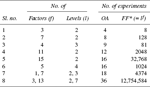
*Number of FF is lf where l is the number of levels and f number of factors.
An important observation
Before proceeding further on OA, the authors would like to state that there is a common notion that DOE in general and OA in particular are beyond ordinary capability. This is a mistaken view. It is the experience of authors that OA has been learnt and applied by many satisfactorily. The methodology has to be put across a practical-do-it way rather than using statistical jargons. The same thought applies to statistical techniques dealt in Chapters 23 and 24. Knowledge of OA is compulsory for anyone involved in continual improvement.
Understanding OA design
Consider the OA design, L8 (27), as shown in Figure 25.1.
The following properties that can be observed are those of the experimental design called L8 array being balanced and orthogonal.
Figure 25.1 OA design L8 (27)

Note: It is not essential to know the basis of ‘how’ of the design and its linear graph, the same way as to how the calculator functions for its user.
- The number of levels of (1) and (2) in any column is the same.
- The number of levels of (1) and (2) found in any column is the same for each column.
- The property in (ii) is true of every two columns in the array.
- Let each column be assigned to each of the seven factors A, B, C, D, E, F and G; each factor has two levels (1) and (2) represented as (A1, A2), (B1, B2), etc., and the yield (response) from each experiment Y1, Y2, etc., as shown in Table 25.2.
TABLE 25.2 Factors, Levels and Response of Each Experiment
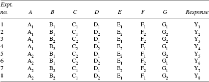
From the table notice the following results.
Y1 + Y2 + Y3 + Y4 = 4A1 + 2[B1 + B2 + C1 + C2 + D1 + D2 + E1 + E2 + F1 + F2 + G1 + G2]
Y5 + Y6 + Y7 + Y8 = 4A2 + 2[B1 + B2 + C1 + C2 + D1 + D2 + E1 + E2 + F1 + F2 + G1 + G2]
From the results, the following observations can be made.
Response of A at the level A1 is influenced by each of the levels B–G.
Response of A at the level A2 is also influenced by each of the factors B–G.
This is due to the property of orthogonality. It can be verified that the same holds good for B–G.
Now the difference in the sum of yields shown here measures the effect of A on response by changing it from level A1 to A2.
A1 − A2 = ¼ [(Y1 + Y2 + Y3 − Y4) − (Y5 + Y6 + Y7 + Y8)]
This effect is reliable as it is influenced by each level of B–G.
Similar results follow for each factor B–G. Thus, the advantage of FF experiment is derived even when the number of experiments is reduced.
Standard OA designs and their linear graphs
The associated standard linear graphs (SLGs) for standard OA designs are
- Two-level OAs (each factor has two levels):
L4 (23), L8 (27), L12 (211), L16 (215), L32 (231)
- Three-level OAs:
L9 (34), L18 (21, 37), L27 (313)
- Other types of OAs:
L16 (45), L25 (56), L36 (211 × 312), L36 (23×313),
L50 (21×511), L54 (21×325), L64 (263), L64 (421), L81 (340)
As an explanation, L4 (23) means that a minimum of four experiments are to be conducted when the number of factors and interactions to be assessed is 3 or less and two levels are involved. Similar interpretation holds good for all such designs.
Steps in designing, conducting and analysing an experiment
The steps involved in designing, conducting and analysing the data and follow-up action are as follows.
- Selection of factors and/or interactions to be evaluated.
- Selection of number of levels for the factors.
- Selection of the OA and assignment of factors and/or interactions to columns.
- Conduct experiments.
- Analysis of experimental results.
- Confirm experiment.
Selection of factors
Factors are determined to investigate the hinges on the product or process performance characteristic(s) or response(s) of interest. The following tools are useful in identifying the factors.
- Brainstorming
- Flow chart (especially for processes)
- Cause–effect diagrams
Selection of number of levels
In the first round of experimentation, it is better to have three to four factors and interactions thought to be relevant on the basis of knowledge, experience, intuition as well as data backup. It is better to have only two levels for each factor.
This will help to identify the key factors and then get into the next phase of few established factors but at multiple levels for each factor, if necessary.
Selection of OA and assignment of factors and/or interactions to columns
A number of examples have been worked out on the selection of OA and allocation of factors and/or interactions to columns.
Conduct the experiment
All precautions and technical discipline needed are to be followed. The experiments are to be conducted in a random order and not serially as shown in the experimental design layout. A minimum of one test result must be obtained. The number of test results should remain the same for each experiment in case more than one test result is obtained.
Analysis of experimental results
Method of analysis of data is known by the name analysis of variance (ANOVA). This technique has been explained in Chapter 23. Here, two illustrative examples of the analysis of experimental data by ANOVA have been given, one each for variable data and attribute data.
Confirmation experiment
The confirmation experiment is the final step in verifying the conclusions from the previous round of experimentation. Optimum conditions are set for the significant factors and levels and several tests are made. The average of the confirmation experiment results is compared to the anticipated average based on the factors and levels tested. The confirmation experiment is a crucial step and should not be omitted.
Selection of OA and allocation of factors and/or interaction to columns–illustrative examples
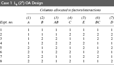
Case 1. Regarding the stability of the power factor of capacitor, it was decided to examine the effect of five factors: (A) leakage current of the foil, (B) power factor of the foil, (C) capacitance value of the foil, (D) soaking time during impregnation, (E) loading pattern—each one at two levels. It was also felt necessary to examine the interactions AB and BC. The levels are A:2 and 3 μA; B: 3 and 5 per cent; C: 8–10 and 11–13 μt; D: 2 and 4 hr; E: 70 and 100 per cent.
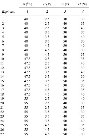
Case 2. Four factors A, B, C and D corresponding to bath temperature, voltage, duration of immersion and concentration of bath, respectively, were considered important to get the required colour in a wristwatch dial. It was decided to assess the effect of each factor at three levels, in addition to the evaluation of interaction effects AB, AC and BC. The levels of each factor are three and they are A: 40, 47.5 and 55°C; B: 2.5, 3.5 and 4.5 V; C: 30, 40 and 50 min; D: 30, 35 and 40 per cent.
Case 3. A, B, C, D and E; BC and CD are the main factors and interactions of interest. The level of each factor is 3 and each is indicated by (1)–(3) for every factor.
For the above three cases:
- Choose the appropriate OA design for each.
- Assign factors and interactions to columns.
- Set up the experimental design matrix.
There is a common step-by-step procedure mentioned in the following context to accomplish the stated tasks.
Step 1: Know levels of main factors and the interactions of interest.
Case 1: A, B, C, D, E each at two levels; interactions AB, BC
Case 2: A, B, C, D each at three levels; interactions AB, AC, BC
Case 3: A, B, C, D, E each at three levels; BC, CD
Step 2: Find degrees of freedom (d.f.) for main factors and interactions.
d.f. main factor = no. of levels − 1.
d.f. interaction AB = (d.f. A) × (d.f. B)

Step 3: Minimum no. of experiments (MNE) = Total d.f. + 1
Case 1: 7 + 1 = 8
Case 2: 20 + 1 = 21
Case 3: 18 + 1 = 19
Step 4: Choose OA design with its number of experiments closest to MNES found in step 3 satisfying the d.f. [Refer the list of OA designs listed as shown and find the appropriate design]
Case 1: L8 (27)
Case 2: L27 (313)
Case 3: L27 (313)
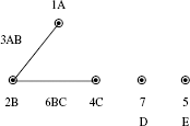
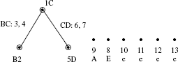
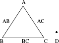
Step 5: Draw the required linear graph (RLG) using the information available in Step 1. Represent by ![]() the main factor and join two such factors to denote the interaction of interest.
the main factor and join two such factors to denote the interaction of interest.

Step 6: Select SLG associated with the OA decided in step (4) and record it next to RLG as shown above in case (1) to (3). [Note: To get the SLG refer book having the serial number (5) in the list of references]
Step 7: Modify the SLG to meet RLG (if it is not possible choose the next higher OA design and repeat the above steps) and indicate the alphabet of the factors in the modified SLG as shown.
Case 1:
Case 2:
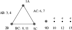
Step 8: Write down the OA design. Note the following in the OA design as well as the modified SLG.
- Levels are indicated by the numerals 1, 2 and 3 to reflect level 1, level 2 and level 3, respectively.
- Columns represent the factors and interactions to be addressed.
- The numerals in SLG refer to the column numbers.
- Thus, in the modified SLG graph arrived at in step 7, the column number and the factor/interaction associated with it are shown. This factor/interaction is allocated to the column number in the OA design.
- If some column numbers remain without any factor/interaction, they are error columns shown by the letter ‘e’.
These points are followed in allocating the factors, interactions and columns in OA design.
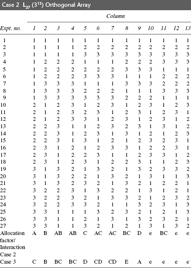
It can be verified that the allocation for case 3 is as above.
Step 9: Write the experimental design matrix and insert the actual values of the levels of each factor leaving out the columns allocated to interactions and e (error). Care must be taken to avoid clerical error by wrong posting of the values of the level.
Case 1:

Case 2: Master plan of the experiment
Case 3: Try working this yourself!
Step 10: Check in step (8) whether any column is allocated for error (e). If not, the entire set of experiments needs to be replicated at least once to obtain an estimate of the error needed for assessing the factor and interaction effects.
Case 1: There is no column for error. Hence, repeat the entire set of eight experiments shown in step 9.
Cases 2, 3: Columns are available for error.
Step 11: Find the random sequence for conducting the experiments—8 in case 1, 27 in case 2, 27 in case 3 and conduct the experiment as per the random sequence and record the response/result of each experiment. For example in case 1, the random sequence can be
Replication 1: 4, 1, 3, 2, 8, 7, 5, 6
Replication 2: 6, 5, 2, 4, 7, 1, 3, 8
Using these sequences, the 16 experiments are conducted and not serially from 1 to 8.
Analysis of experimental results: response by measurement (variable) data—illustrative example 1
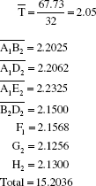
In an investigation to find the best condition of molar ratio for the production of sodium silicate, the following factors with their levels and interactions were chosen for the experiment. Interactions of interest are AB, AD, AE, BD and DE (Table 25.3).
TABLE 25.3 Factors and Levels
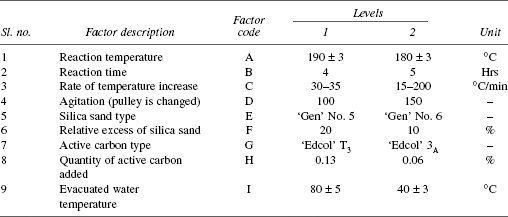
- Find the appropriate design layout.
- In the layout, data on molar ratio are given. Two measurements are taken for each experiment. Analyse the data and obtain optimum combination of factors that increases the molar ratio.
Answer
- The total d.f. is 14: one d.f. for each of A–I totalling 9 and one d.f. each of AB, AE, BD, DE, AD totalling 5.
- MNE 14 + 1 = 15.
- The appropriate OA design is L16 (215); the nearest corresponding MNE is 15.
- The RLG is:

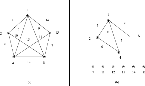
- The SLG is shown in Figure 25.2 (a)
- The modified SLG is shown in Figure 25.2 (b)
Figure 25.2 (a) SLG (b) Modified SLG
- The assignments are as follows: factors to modified SLG.

- The design layout is given in Table 25.4.
Analysis of the data The design layout with the data obtained from the experiments is shown in Table 25.4.
TABLE 25.4 Design Layout and Response for Analysis

(A) Prepare total response (Table 25.5) for the main factors/interaction.
TABLE 25.5 Total Response Table for Main Factors and for the Columns of Interactions/Errors

*Total being the same for each of the factor is a cross-check on the correctness of the calculation.
(B) Total response table for interactions (Tables 25.6–25.10).
TABLE 25.6 For Interaction A × B

TABLE 25.7 For Interaction A × D
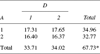
TABLE 25.8 For Interaction B × D
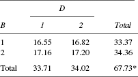
TABLE 25.9 For Interaction D × E

TABLE 25.10 For Interaction A × E

*Total being the same in Tables 25.6–25.10 is a cross-check on the correctness of the calculation.
(C) Sum of the squares calculation
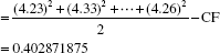
- Correction Factor (CF) = (67.73)2÷ 32 = 143.355
- SA = sum of the squares due to Factor A

Note. To find out the sum of the squares of a factor having two levels, the formula (A1 − A2)2/n can be used; where Ai = sum of the observations when the factor A is at level ‘i’, i = 1, 2; and n = total no. of observations.
Thus, - SB = 0.030628125 (d.f. = 1)
- SC = 0.000028125 (d.f. = 1)
- SD = 0.003003125 (d.f. = 1)
- SE = 0.136503125 (d.f. = 1)
- SF = 0.052003125 (d.f. = 1)
- SG = 0.002628125 (d.f. = 1)
- SH = 0.005778125 (d.f. = 1)
- SI = 0.000153125 (d.f. = 1)
- SA × B = 0.005778125 (d.f. = 1) = sum of squares due to interaction A × B (d.f. = 1)
The sum of the squares of interaction between A and B can also be found out by using the cell total of the two-way table for interaction A × B.
i.e.,

- SA × D = 0.004278125 (d.f. = 1)
- SA × E = 0.010153125 (d.f. = 1)
- SB × D = 0.001653125 (d.f. = 1)
- SD × E = 0.000378125 (d.f. = 1)
- Sel = Sum of the squares due to column 15 which is free in the layout of the design
= 0.000028125 (d.f. = 1) - ST1 = Sum of the squares due to the ‘16’ treatments (which are the combination of different levels of the factors A, B,…, G, H)
- ST2 = Total sum of squares
= (2.11)2 + (2.12)2 + (2.16)2 + … + (2.12)2 + (2.14)2−CF
= 143.7617 − CF = 0.40692188 - Se2= Error sum of squares due to replication
= ST2 − ST1
= 0.004050005
(D) ANOVA table is given in Table 25.11.
TABLE 25.11 ANOVA Table

Note: MS (Mean Square) is obtained by dividing SS from d.f. SS stands for sum of squares and d.f. for degrees of freedom.
e1 and e2 are pooled to get e1 for d.f. and SS as MS e is less than that of e. e1, C, and I are pooled to get e11 for d.f. and SS as MS of each of C and I is less than that of e1. e11 and DE are pooled for d.f. and SS to get e111 as MS are not statistically different. Fcal corresponds to the ratio of MS of all factors and interaction except C, I and DE compared to MS with e111. C and I are pooled because the MS is not statistically significant.
Nearly 90 per cent of the total SS of ST1 is explained by the significant factors and interactions. This is an indication that appropriate factors have been included in the experiment.
(E) Prepare Tables 25.12–25.16 corresponding to the average response table for the main factors and interactions that are found statistically significant.
(F) The optimum combination is A1 B2 D2 E2 F1 G2 H2, based on the scrutiny of Tables 25.12–25.16.
TABLE 25.12 Average Response Table for Significant Main Factors
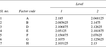
TABLE 25.13 For Interaction A × B
| A | B | |
|---|---|---|
| 1 | 2 | |
| 1 | 2.1675 | 2.2025 |
| 2 | 2.00375 | 2.0925 |
TABLE 25.14 For Interaction A × D
| A | D | |
|---|---|---|
| 1 | 2 | |
| 1 | 2.16375 | 2.20625 |
| 2 | 2.05 | 2.04625 |
TABLE 25.15 For Interaction A × E
| A | E | |
|---|---|---|
| 1 | 2 | |
| 1 | 2.1375 | 2.2325 |
| 2 | 1.965 | 2.13125 |
TABLE 25.16 For Interaction B × D
| B | D | |
|---|---|---|
| 1 | 2 | |
| 1 | 2.06875 | 2.1025 |
| 2 | 2.145 | 2.15 |
(G) Estimate the mean for the treatment combination, μA1 B2 D2 E2 F1 G2 H2
where interactions are A1B2, A1D2, A1E2 and B2D2:
where the coefficient of the term T (overall average) is one less than the number of items added to estimate the mean:
Therefore, μA1 B2 D2 E2 F1 G2 H2 = 15.203−12.300=2.9036
It can be observed that the average of 2.90 corresponding to the optimum combination is higher than any of the other average values.
(H) Confidence interval
Confidence interval for the predicted treated condition is as follows:
where

Significant factors are A, B, D, E, F, G, H and interactions are A1B2, A1D2, A1E2, B2D2

In the confirmation experiments the factor combination to be used is A1 B2 D2 E2 F1 G2 H2.
Analysis of experimental results: response by attribute data—illustrative example 2
Response from an experiment is not a measurable characteristic, but an ‘attribute’ whether a desired feature is present or not. If the desired feature in an item is present it is OK, otherwise Not OK.
Four factors A, B, C and D and the three levels considered for each factor are given in the following table. Interactions AB, AC and BC are considered important grounds of opinion.
Factors and levels
Selection of design layout
- Total d.f. = d.f. of main effects + d.f. of interactions
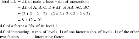
- Minimum no. of experiments = 20 + 1 = 21
- Standard design to ensure minimum no. of experiments subject to (ii) is L27 (313)
- RLG is
- SLG associated with L27 (313) is

- Modified linear graph. The first one is more suitable to the RLG. The modified version of the first SLG is
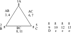
- The design layout regarding the allocation of columns is as follows. This helps in data analysis.
- Experimental layout inserting the levels of factors are as follows. This is as per L27 (213).
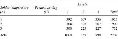
- Response data were obtained as follows:
- For each experiment, 3 PCBs were wave soldered.
- The total no. of joints in each PCB was 462.
- Response considered: number of joints with blow-hole as a defect. Data on no. of joints with blow-hole were taken as response. Thus, the following points arise:

Total no. of joints per level per factor = 9 experiments per factor per level × 3 PCB per experiment × 462 joints per board = 12,474 for each of A, B, C, D
Total (response) no. of defects over 27 experiments = 2707
In the experiment layout table, response data of experiment—number of blow-holes in each of the three PCBs—are posted for each of the 27 experiments. Thus, the results mentioned follow from these details.
- Total no. of PCBs is = 27 × 3 = 81
- Total no. of joints in each factor combination = 462 × 3 = 1386
(No. of items checked) - Total no. of joints for 27 experiments = 462 × 3 × 27 = 37,422
- Total no. of blow-holes found = 2707
Response summary data
Prepare the following response summary data
- Main factor A, B, C, D for each of its three levels.
- Interaction response summary table of each level of a factor corresponding to each level of the other.
These are given in Tables 25.17–25.20.
TABLE 25.17 Total Response Table for Main Factors

*No. of observations for each level of the factor = 12,474.
**No. of observations for a factor for three levels overall = 37,422.
TABLE 25.18 Total Response Table for Interaction A × B

*No. of observations for each combination of a level of this factor is 4158 (3 × 3 × 462)—3 experiments with same levels, 3 boards per experiment and 462 joints per board.
TABLE 25.19 Total Response Table for Interaction B × C
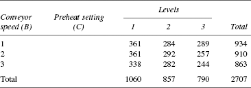
TABLE 25.20 Total Response Table for Interaction A × C
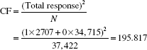
Correction factor
Total number of observations made in the 27 experiments are as follows:
- Total no. of joints inspected (N) = 37,422
- Total no. of defects found = 2707
- Total no. of non-defects = 34,715
- Assigning a score of ‘1’ to defects and ‘0’ to non-defects, the total response from 37,422 numbers inspected is = 2707
Sum of squares


Analysis of variance table
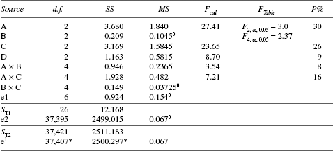
*e1 is the pooled d.f. and SS of e1, e2, factor B and interaction B × C.
Fcal is the ratio of MS of each source except B and B × C with the MS of e1.
Summary of results—average response of significant factors and interactions

Optimum combination is A3 B3 C3 D2
Average no. of defects for the optimum combination is
(It can be verified that the combination A2 B1 C3 D2 is inferior to A3 B3 C3 D2)
Therefore, the average present level of 7.3 defects per 100 joints would get reduced to 2.8 per 100 joints.
95% confidence interval is given by ![]()
where v1 = 1, v2= d.f. of MSe = 37,407(∞), MSe = error variance = 0.067, neff = effective d.f. and α = 0.05
Thus,
Fv1, v2, α = F1, ∞, 0.05 = 3.84
Therefore,
In the confirmation experiments, the factor combination to be used is A3 B3 C3 D2.
Conclusion
Knowledge of continual improvement process, statistical tools and techniques of analysis can be of good and effective use only when continual improvement task is well organised as a managerial function. Thus the next Section F deals with the managerial aspects of organising continual improvement.
Annexure 25A
Comparison between conventional and statistical methods of experimentation
Note: Comparison of the two approaches given is as applied to an experiment with two factors. The same conclusions hold good for an experiment with more than two factors.