
CHAPTER 12
Basics of Six Sigma Technique
The greater danger for most of us is not that our aim is too high and we miss it, but that is too low and we reach it
– Michelangelo
SYNOPSIS
In this chapter, system control on defects is explained. When system approach ceases to be effective, process approach takes over to reduce defects. This aspect is clearly explained. A process does reach ‘zero’ defect level when its variability is far less than what is permissible by specification. This key point is explained and illustrated. A new process parameter z, the Sigma of the process, is developed along with another entity, first time yield (FTY). The essence of Six Sigma technique are z and FTY. A large number of examples have been worked out to make one familiar with the use of Six Sigma technique. A number of areas of application of Six Sigma technique have also been dealt with.
Background
It is becoming a common practice for companies to develop and put in place a comprehensive quality system on the basis of international standard ISO 9000:2001 and also seek certification for the system under ISO 9000:2001. Such a practice leads to a proper housekeeping system; control of instruments and gauges; control of tools, jigs and fixtures; proper identification, storage, handling of items, etc. When such systems are in place and implemented efficiently, it yields good, faster results as stated in Table 12.1.
Once the system gets established and updated regularly, the results stabilise and the rate of improvement tapers off. But the pressure of customers demanding better levels of quality and service mounts without respite. Refinement in the system does not contribute much. This is the time when most of the companies launch varieties of technique-oriented, motivational and behavioural programmes such as Kaizen, Quality Circles, Total Productive Maintenance and Failure Mode Effect Analysis to improve the quality level. These do contribute to enhance performance and it gets stabilised at improved levels. At this stage, the feeling of not having much of a scope to improve the results sets in.
It is at this point of time the thought of elimination of defects/errors/non-conformance should reach out to individual micro operations. This is process approach. In this approach, the logic of elimination of defects in a process runs as follows:
TABLE 12.1 Type/Class of Defects Prevented by Systems (Illustrative) in a Manufacturing Organisation
| Particulars of defects prevented by systems |
|---|
Defects that arise because of using
|
| Issue of purchase orders with errors |
| Acceptance of order not possible to execute |
Defects due to
|
| Wrong dispatch |
| Short dispatch |
- Is the process doing its best? Answer to this question lies in examining the question, ‘Is the process under statistical control?’
- If the process is not in statistical control, take actions to bring it under statistical control.
- If the process is in statistical control, does it assure that the output complies with the specification/required tolerance such that the rate of failure/defects is at 3.4 ppm Six Sigma level.
- If not, take action to minimise the process variation to meet the Six Sigma level of performance. This thought of minimising variation in a process is enhancing the very capability of the process, through maintenance based on condition monitoring, feeding more homogeneous control, environmental control where required, control on process interferences and technology upgradation.
Thus, process approach has as its focus elimination of defects/errors/non-conformance so as to reach the near-zero level of 3.4 ppm termed as Six Sigma level. These aspects of the logic stated above are discussed in the subsequent sections of this chapter.
Thought process of Six Sigma
It is explained later in this chapter that the tool of Six Sigma approach provides two parameters for each process—first time yield (FTY) and z value measure of FTY of the process and the inherent capability of the process (z value) corresponding to its defect level. They help in prioritising the processes for improving their capability through planned action. Six Sigma is essentially an exercise in improving the process, its capability and thus reducing the defects to ppm level to reach the ideal of 3.4 ppm (Six Sigma status).
Six Sigma is a statistical tool. It is a remarkable tool as it has opened up the path to (a) reach zero defect level and (b) assess each process and specify how close it is to the ideal level. It is also remarkable in the sense that the mechanics of applying the tool is easy and simple.
Process, quality characteristic and specification
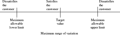
A process is a set of operations carried out by utilising resources to turn out a desired output. The resources of an operation that drives it to turn out an output are the four M’s—man, machine, method and material. The output has to meet certain features. These features are specified and they are called quality characteristics. Each quality characteristic has to comply with certain stated specified requirements. These are called by the generic name specifications. When the requirements stipulated in the specifications governing every quality characteristic of the output are completely met for each quality characteristic, the process meant for producing the output is said to be satisfactory. Otherwise, it is not. This point is illustrated in Figure 12.1.
Figure 12.1 Quality characteristic and specification
Specification, variation, process capability
Specification for a quality characteristic indicates the limits within which the value of that quality characteristic can be. For example, if the length of a bolt is stated as 1 cm, the entire output of bolts cannot have the same length as 1 cm; the length does vary from piece to piece. Hence, a limit is specified for the length like 1.0 ± 0.1 cm, whereby all the bolts having their length within the stated bandwidth termed ‘specification’ are acceptable. Specification is determined on the basis of technical considerations as well as customer requirements. Specification is imposed on a process and the process has to comply with it. Another important feature of specification that has to be recognised is that specification represents the permissible limits of variation from target value. In the example cited above, 1.0 cm represents the target value and ±0.1 cm represents the permissible variation from the target value.
Quality characteristic when measured on the output of a process shows that measurements vary from one piece to another and are not identical. This is true for any parameter of a process. This is the variation from the process. Hence, any process is statistical in nature. The variation from the process has to be quantified to judge the ability of the process to comply with the specification. Quantification of variation in a process is a statistical exercise. Variation quantified is called Sigma and it is normally designated by the symbol ‘σ’ or ‘s’ or ‘s.d.’
Process capability and quality system
Process capability is a measure of variation in the process. Specification is a measure of variation that is permitted in the product, which is the process output. Thus, the relationship that process capability bears with specification is at the very root of output complying with its specification. Product not complying with specification is a defect/non-conformance. Hence, process capability answers whether a process is inherently capable of being defect-free. In case the process capability is superior to specification, the output meets the requirements fully and hence defects/non-conformance does not exist—Six Sigma level is achieved. These aspects are discussed in the subsequent sections of this chapter.
Process capability (PC), a measure of the variation in the process, is defined as
PC =±3σ or 6σ
The basis of PC as equal to 6σ lies in the logic of statistical process control and this is explained in the next section on the basis of statistical law called Normal Law.
Presently, it is to be noted that the ability of a process to meet the specification lies with its PC. If PC is superior to the specification, then it is possible to comply with the specification.
Interrelationship between quality system and PC is shown in Table 12.2.
TABLE 12.2 Quality System and Process Capability
| Quality system | Process capability |
|
|---|---|---|
| Inferior | Superior | |
| Inferior | Worst Focus on setting right the system |
Potentially excellent but rendered inefficient Priority: setting right the system |
| Superior | Potentially excellent Improve process capability |
Super excellent Maintain system and process capability in super state |
Statistical control
A process is performing at its best when it is under ‘statistical control’. A process under statistical control means variability found in any aspect of the process under study, like quality characteristic, yield rejection and defect, is consistent in complying with the underlying statistical laws. When the quality characteristic is a measurable one, the statistical law that governs its variation is ‘Normal Law’ which is explained in the next section.
Figure 12.2 explains the concept and logic of statistical control. From Figure 12.2, it can be seen that
- Variability due to special causes that disturbs a process has to be eliminated keeping in place effective systems. This is the phase of restoration already explained in Chapter 3.
- Variability inherent in the process has to be reduced so that it is superior to specification by a factor of minimum 1.5 to touch near-zero defect level of 3. 4 ppm. This is the phase of ‘breakthrough’ explained in Chapter 3.
Figure 12.2 Flow chart on process and variability in the process

Thus, (1) and (2) together constitute the task of continual improvement that binds a process.
Normal law
The concept of normal law can be easily conceptualised as follows.
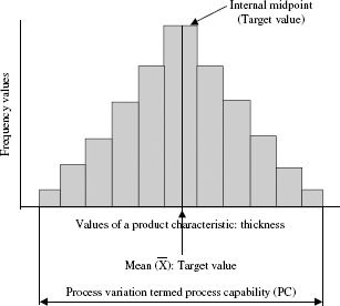
Any measurable quality characteristic has to comply with the specification allowed. For example, if the thickness of a strip is 1 mm and allowed limits are ±0.05 mm, then the target value is 1 mm, and allowable maximum and minimum limits are 1.05 and 0.95 mm, respectively.
Manufacturing process is geared to produce at the target value. Thus, the number of measurements peaking at the target level and tapering off on either side of the target value are depicted in Figure 12.3. This is the pattern of normal law.
Figure 12.3 Pattern of normal law
In Figure 12.4, standardised normal law free from the unit of measurement applicable to any quality characteristic is given. In this standardised version, target value is 0 and Sigma is 1.
Tables giving area under the normal law are available in any standard book on the subject of statistics. From these tables, the areas enclosed at a distance of ±1σ, ±2σ, ±3σ from the target value of ‘0’ can be read. It can be seen in Figure 12.4 that 99.73% of the output lies within ±3σ. It is for this reason that PC is defined as ±3σ.
Thus, when a process is centred at the target value and variation in the process is random and not due to special causes, 99.73% of the output is covered by ±3σ PC. It is the minimum variability that has to be tolerated due to random variation. If specification limits coincide with ±3σ PC, then non-conforming output is 0.27% or 2700 ppm.
Figure 12.4 Generalised normal law and process capability

Specification, process capability, defects and key thoughts of Six Sigma technique
A clear understanding of the relationship between specification, process capability and defects indicates the route to achieve the Six Sigma level of near-zero defects status. This understanding can be developed by examining the Figure 12.5, where
- The letter ‘T’ stands for target value of any quality characteristic.
- The letters ‘U’ and ‘L’ stand for the upper and lower specifications, the permissible limits of variability.
- Bell-shaped curves represent the process under a state of statistical control.
- Process variability being far greater than permissible limits shown in (A), (B); process variability just matching the permissible limits in (C); process variability being far superior to permissible limits in (D).
- Defects status corresponding to A, B, C and D is indicated for each case.
Following observations can be made from Figure 12.5.
- Defects are those that are beyond specification.
- Defects occur when the PC is beyond the specification limits, upper as well as lower.
- Defect in case (B) is reduced compared to case (A); defect in case (C) is reduced compared to case (B); and defect is almost zero in case (D). This is due to the base of the curve (PC) getting narrowed. In other words, PC is getting reduced.
- Hence, an effective tangible route for defect elimination is continuous improvement in PC, numerically reducing the variation. This is the tool of Six Sigma.
Figure 12.5 Process, target value, upper and lower specification limits, defects

Thus, the key result area through the tool of Six Sigma is given as
Eliminate defects through reduction in variability.
Process capability and Sigma value of the process
It becomes necessary to assess first the prevailing capability of a process. This assessment can be made on the basis of the existing defect rate of the process. Defect rate can be assessed on the basis of defect data obtainable from the process. Thus, the question that arises is how to assess the PC based on defect rate? To facilitate this, the entity Sigma value of the process denoted by z is derived as under.
The term PC index is defined as follows and it indicates the relationship between specification and PC. PC index is denoted by Cp.
where U and L are upper and lower specification limits.
In other words, ![]() , where Cp stands for PC index.
, where Cp stands for PC index.
The given equation is such that when the process variability (6σ) decreases, the value of Cp (the PC index) increases. From Figure 12.5, it can also be noted that defect progressively touches zero with increase in PC index from 0.33 to 1.66.
Now, ![]() , where
, where ![]() and
and ![]() are the target values.
are the target values.
Therefore, ![]()
Define ![]() as Sigma value of the process (z) with the provision U can be a general value like x.
as Sigma value of the process (z) with the provision U can be a general value like x.
Therefore, ![]() or z = 3 Cp.
or z = 3 Cp.
When z = 3Cp, z cannot be negative, since U > L. z ranges from ‘0’ and upwards. Since z is linked to Cp, the PC index, z value is called the ‘Sigma value of the process’. The method of determining z value is through defect rate as explained in the next section.
Obtaining the Sigma value of a process: z value from defect rate
Tables 12.3 and 12.4 are used to obtain the Sigma value of the process from defect rate.
- The tables give the defect rate as proportion.
- The defect rate corresponding to different values of z can be found from the table and the following statements can be verified.
For z value of 1.31, the defect rate is 0.0951.
For z value of 2.33, the defect rate is 0.00990.
- From the defect rate, the corresponding values of z can be found from the tables and the following statements can be verified.
For a defect rate of 0.01072, the corresponding z value is 2.30.
For a defect rate of 0.000577, the corresponding z value is 3.25.
TABLE 12.3 Single-Tail z Table—Values of z from 0.00 to 3.99

TABLE 12.4 Single-Tail z Table—Values of z from 4.00 to 5.90

Note: z value in the table is equal to 3Cp where Cp is the PC index. This point needs to be noted while using the table based on Cp values.
Defect rate has to be in terms of defects-per-opportunity (DPO) and DPO can be expressed as DPMO (defects-per-million-opportunity) (ppm at opportunities level). The various points to be noted for capturing the defect data have already been discussed in Chapter 4.
z Table and its use
Tables 12.3 and 12.4 give the values of z corresponding to different values of defect rate expressed as DPMO. The use of this table in determining the z value of a process is explained in the illustrative examples.
For a process, where defect data can be captured in terms of the number of different types of defects that can occur in a process, FTY and z values can be determined as quality measurements of a process.
Illustrative examples: calculating z value from defect data
Illustration 1
There are five processes, A to E. Data on number of units inspected, number of defects found and number of types of defects (number of opportunities) in each processes are given. Method of obtaining the z value of each process is also illustrated in Table 12.5.
TABLE 12.5 Calculation of z Value

TOP: Total number of opportunities = u × m
DPU: Defects per unit = D/u
DPO: Defects per opportunity = D/u × m
DPMO: DPO × 106 = D × 106/(u × m)
*Locate the value in the body of Tables 12.3 and 12.4.
**Read the corresponding value of z, the Sigma value of the process.
Illustration 2
Find the z value and process capability for the following defect rate as ppm: 3.4, 58, 277, 1390, 1845, 4600, 2540, 22,881. Comment on the results. Calculations are set out in Table 12.7.
Process categorisation as per its Sigma value is given in Table 12.6.
TABLE 12.6 z Value and Process Categorisation

*Six Sigma level company value.
TABLE 12.7 Defect Rate, z Value, Cp Value
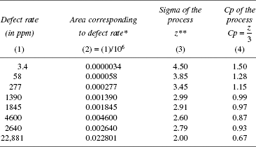
*Locate the value of the area in the body of Tables 12.3 and 12.4.
**Read the corresponding value of z, the Sigma of the process.
Following are the comments.
- The Sigma value of the process (z) decreases as the defect rate increases.
- The Sigma value of 4.5 is the goal for any company aspiring to be a Six Sigma company and it corresponds to the defect rate of 3.4 ppm.
- Therefore, the objective of Six Sigma for any process is to attain a Sigma value of 4.5 by effective defect prevention measures.
- Process capability of a process is its Sigma value (z value) divided by 3. This is a simple method of arriving at PC based on defect data. Thus, defect data is the key in Six Sigma analysis.
First time yield (FTY)
Classical definition of FTY is discussed in Illustration 3.
Illustration 3
One hundred units are inspected and 10 units are not passed (which are defective).
Next issue relates to the 10 numbers not passed. What are the defects for which they were not passed? A unit not passed can have one or more defects. Hence, the number of defects can exceed the number of units not passed.
As against the classical definition of FTY, there is the approach to find FTY based on statistical law called Poisson distribution and with this it would also be possible to predict the proportion of defect-free output from a process. These are dealt in Illustration 4.
Illustration 4
One hundred units are inspected after production. Number of units passed is 90. The number of defects found among the 10 units not passed is as follows.
On the basis that the defect per unit (DPU) is 1.0, is it possible to predict the proportion of output that is defect free?
It is possible on the basis of the Poisson’s law, which postulates

For example, DPU = 1.0; therefore, FTYd = e−1.0 = 0.3678. That is, 36.78% or 37% of the output is defect-free. Thus, process capability is inadequate even when it is in a state of statistical control as 37% of the output does not meet the specification.
Thus, it can be noted that in the classical approach where defects are not taken into account, predicting the defect-free output is not possible and thus no understanding of the inherent capability of the process is possible.
Thus, FTY is another performance metric of a process that estimates the defect-free output on the basis of the existing DPU. To get the correct FTY, it is important to have database on defects which are complete and correct.
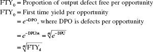
First time yield and z value
FTYd = e–DPU, where DPU is the defect rate per unit.
DPO Defect per opportunity = ![]() , where ‘m’ is the number of opportunities.
, where ‘m’ is the number of opportunities.
‘m’ is the number of opportunities that are there for a defect to occur. It can also be taken as the different types of defects that can occur. For example, in a process where five types of defect can occur, the value of ‘m’ is 5. This is not same as number of defects that has occurred which can even be zero or much more than the number of opportunities available. This distinction needs to be noted to avoid confusion between number of defects occurred and number of types of defects that can occur.
Like FTYd, FTY0 can be defined as
z is Sigma value of the process from Tables 12.3 and 12.4, corresponding to the proportion of output with 1 or more defects when defect rate is DPO.
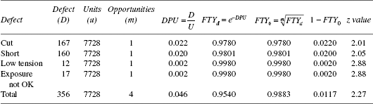
Illustration 5
During the period July 2001 to October 2002, among 7728 stencils, the number of defects found are: cuts, 167; short, 160; low tension, 12; exposure not OK, 17.
Find the Sigma value as well as FTY related to each type of defect.
| Total no. of stencils inspected | 7728 | |
| Types of defects | ||
| Cuts | 167 | |
| Shorts | 160 | |
| Low tension | 12 | |
| Exposure not OK | 17 | |
| Total no. of defects | 356 | |
| No. of opportunities per stencil | 4 | |
Layout for calculation
Rolled throughput of a process
Illustration 6
For the example given in Illustration 4, obtain FTY for each defect.

*FTY of the process where defects A, B, C, D and E occur is called rolled throughput and it is obtained as follows.
FTY of the process = FTYA × FTYB × FTYC × FTYD × FTYE × = e−ΣDPU = e−1.0
= 0.3679 or 37%
Comments on the analysis presented above are
- FTY related to each defect contributes to the overall FTY of the process.
- For maximising FTY of the process, FTY of each defect has to be maximised.
- FTY gets maximised when DPU gets minimised.
- DPU gets minimised when the defect rate for each type of defect gets reduced.
- A defect reduction plan specific to each defect type has to be in place.
- This type of analysis needs to be carried out once in a month and defect reduction plan needs to be reviewed to render it focused and effective.
- Database which provides for capturing all the different types of defects is a prerequisite.
- While collecting the data on defects, all the defects found in the item not passed need to be recorded. The commonly found practice of stopping inspection of an item on finding a defect and recording as not passed and then proceeding for the next item does not serve the purpose.
Illustration 7
Obtain FTY of each process, Sigma value for each process and estimate the FTY for the entire sequence of eight processes (database provides for capturing all the defects (m) item-wise).
Product of the FTY of each process involved in the output of a product is the overall rolled throughput of the manufacturing process of the product.


FTY of the entire sequence of eight operations = Rolled throughput over the eight operations
= FTYA × FTYB × FTYC × FTYD × FTYE × FTYF × FTYG × FTYH × e−ΣDPU
= e−0.00385 = 0.99615 or 99.62%
Illustration 8
For each process step, find its FTY and z value.

Note: If the data captures the number of defects in each type of defect, DPU can be found and corresponding FTY for each defect can be computed.
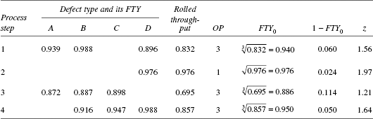
Illustration 9
In Illustration 8, find for each defect in z value.

Illustration 10
Combine the results of Illustrations 8 and 9 and interpret.

A note on m, opportunities for defects
The meaning of ‘m’ is already explained. The value of ‘m’ has a bearing on the value of z. Hence, one should be judicious in choosing the actual value of ‘m’. This issue is explained through an illustration.
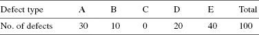
Consider the following example on defects in a loan application.
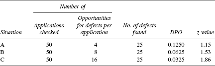
The important point to be noted from the given illustration is as follows.
Is C better than A and B? It is on the basis of their corresponding z values. In reality, C may not be superior to A or B. C has a higher z value than that of A because the value of m used in C is higher than that in A. Therefore, comparison of z values is valid only when the values of m in each z value are same. This validity factor needs to be noted. Consider the following example.

The z value of A is superior to that of B due to the fact that the value of m, the number of opportunities for defects, is higher in A compared to B. This reflects the importance of deciding on the value of m.
Thus, this example indicates that the number of opportunities needs to be reviewed, scrutinised and kept to a bare minimum and this minimum number should reflect the needs of the customer as well as process problems on hand. A higher value of z based on a higher value of ‘m’ gives a misleading information that the process is good, when in fact it may not be so.
Sustainability of improvement
The concept of sustainability of improvement that stems from the technique of Six Sigma method of analysis can best be illustrated through an example given here.
In a certain chemical process, the yield is 95 per cent. A study was conducted to improve the yield. Factors bearing an influence on yield were identified; the levels appropriate for getting an enhanced yield were found by DOE and many batches were produced with revised levels. The yield improved to 97 per cent. As per the conventional practice, the points noted are (a) the improved yield, (b) the duration over which it is obtained and (c) the financial benefit of the 2 per cent increase in yield.
There is no answer to the question about the confidence we can have on the sustainability of the result. In other words, the degree of improvement achieved in the inherent capability of the process to sustain the improvement level of 97 per cent is not known. This void is answered in Six Sigma analysis as follows.
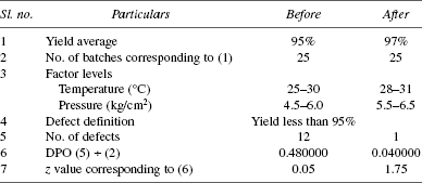
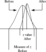
The improvement in the Sigma value of the process (z) from 0.05 to 1.75 reflects the sustainability of the result. Suppose the number of batches with yield less than 95 per cent was to be 8 instead of 1, the corresponding value of z would have been only 0.47 signifying a marginal improvement in the capability. Thus, Six Sigma analysis provides a new insight into the improvement of the capability of the process itself to sustain the improved level which is depicted in the model (Figure 12.6).
First time yield and z value of a process chain
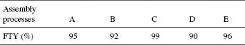
If five individual processes constitute a process chain of A, B, C, D and E, then what are the FTY of the process chain of the five processes and its z value?
FTY of a process chain is the product of the FTYs of individual processes of the chain. This is the YR, the rolled process yield. We know FTY = e−DPU. Thus, FTY of the chain of five processes is
Figure 12.6 Process model for evaluation through Six Sigma
YR = FTY1 × FTY2 × FTY3 × FTY4 × FTY5 × = ![]() = e–[Sum of DPUs] (A)
= e–[Sum of DPUs] (A)
DPOi = Defect at opportunity level in the ‘i’th process = ![]() (B)
(B)
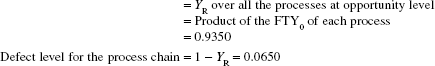
Designating YR0 as FTY at opportunity level for the process chain, by analogy to (A) and (B) above, the following results are obtained.
YR0 = FTY of chain at opportunity level
Defect level for the process chain at opportunity level = 1 – YR0. For the defect level, obtain the value of z from the z table. This is the Sigma value of the process chain. Exercises 8 and 9 in Annexure 12A help to understand the calculations.
Application of Six Sigma tool
Five applications are given.
Illustration 11
Rewinding of burnt motors is mentioned in Chapter 6.
On the basis of the format in Table 6.1, data on defects in the process of rewinding of burnt motors were obtained for 200 motors during the period July–December 2002. The data, thus obtained, are summarised in Table 12.8 which facilitates Six Sigma analysis. From this, follows the Six Sigma report in Table 12.9.
Illustration 12
Customer feedback: outpatients is discused in Chapter 6.
On the basis of the format in Table 6.3, data on feedback were obtained from 100 patients selected at a random of 4 per day over 25 days, Monday through Friday. The data thus obtained is summarised in Table 12.10 which facilitates Six Sigma analysis.
TABLE 12.8 Summary of Data on Rewinding of Motors and Six Sigma Analysis


TABLE 12.10 Summary of Response (No. of Responses: 100)

From Table 12.10, it was noted that the following areas, arranged in the order of priority, need to be examined to start with, to improve the services for the outpatients.
- Interaction with consultant
- Delay in reports—support services
- Waiting comfort
This next phase of the continual improvement project dealing with analysis, implementation and control is discussed in Chapter 27.
Illustration 13
Report on quality: Six Sigma way
In a PCB manufacturing company, defect data were organised in such a way that it facilitated Six Sigma analysis. There is provision to get online summary of the data every day and also prepare monthly report on quality as per Six Sigma. Different stages of this exercise are illustrated here:
- Summary of defects found in 14,960 boards inspected during a 2-week period is given in Table 12.11.
- Summary of FTYs as per defect is given in Table 12.12.
- Summary of process FTY and z value is given in Table 12.13.
- Six Sigma report to management is given in Table 12.14.
It is worth taking up as a project to evolve a system of reporting on quality in terms of process FTY and z value. This truly reflects the improvement in the health of each process by reflecting their z values.
TABLE 12.11 Summary of Defects

TABLE 12.12 Summary of FTYs as per Defect

No. of units inspected (u): 14,960
TABLE 12.13 Summary: FTY and Sigma Value

Process FTY is the product of the FTYs of each defect associated with the process.
TABLE 12.14 Six Sigma Analysis Report to Management (6 to 13 January 2003)
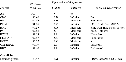
Illustration 14
Facility planning for testing, analysing defective items and their repair
Process of inspection and testing, analysing defective items and their repair is depicted in the process flow chart in Figure 12.7. The data available are also given in the flow chart.
Based on these, assess the present level of output and find the additional equipment, if any, required to meet a uniform output of 10 units/hr from inspection and testing, analysing defective items and their repair. All these timings are based on past performance.
Figure 12.7 Flow chart of inspection and repair

Assessment of cycle time
Cycle time, as its very name, indicates the time taken to complete a specified activity. Shorter the cycle time, higher is the output and vice versa. Hence, the analysis of cycle time is a key element in productivity improvement exercise. Besides this, examination of cycle time of interrelated activities helps to take suitable action on balancing the entire line of production and thus step up the output of the line. These aspects are illustrated with the help of cycle time for inspection (CT. I); cycle time to analyse defectives (CT. A); and cycle time for repair of defects (CT. R) regarding which data are presented in Figure 12.7.
Cycle time of inspection and testing (CT. I):
CT. I = Number of inspections per accepted item × time per inspection and testing
=[2–e–DPU]×Time per inspection
Note on the number of inspections per accepted item
Let the lot size be N. Each item has to be inspected once. Thus, the number of inspections to be done is N.
Items found defective—one or more defects per item—are to be inspected again to take up analysing and repair.
Items found defective is N(1 – e−DPU), where e−DPU is the proportion of output with zero defects.
Hence, the number of second inspection in a lot of N with DPU as defect rate per unit is N(1 – e−DPU).
Therefore, the total number of inspections for the lot of N items to detect accepted items is
N + N(1–e–DPU)
= N[2–e–DPU]
The number of inspections per accepted item is
Cycle time to analyse defectives (CT. A)
CT. A = Workload on analysing × time for analysis
Workload on analysing = DPU, where defect (failure) is analysed one at a time
CT. A = DPU × time for analysis
Cycle time for repair of defects (CT. R)
CT. R = Workload for repair × time per repair
Workload for repairing = DPU, where defect (failure) is repaired one at a time
CT. R = DPU × time for repair
Problem 1
For the flow chart on cycle times in Figure 12.7, output/hour and additional needs of facility to meet an output of 10 per hr are given in Table 12.15.
Following can be verified:
- Additional equipments drop to 2 for inspection and nil for each analysis and repair, when DPU = 0.01 (FTY = 94.6%).
- Additional equipments increase to 4, 20 and 3 for inspection, analysis and repair, respectively, when DPU = 1.00 (FTY = 36.8%).
This again points out the importance of reducing the defect rate (DPU).
TABLE 12.15 Cycle Time Analysis and Facility Assessment

Illustration 15
Planning cell-assembly chain
Cell concept in the manufacture of an assembly has gained wide acceptance as an effective tool to increase productivity through team effort with a focus on achieving the target. The features of cell concept in assembly manufacture are:
- The required target of assembly output per shift is decided.
- The specific distinct processes involved in turning out the assembly are identified. This can include online inspection of semi-assembled units as well as the final assembled units.
- The rate of output of each specific distinct process is assessed.
- The facilities at each specific process—number of machines, equipment, manpower— are geared up to meet the final target of the assembly.
- Each specific process is laid out according to the logic of the assembly processes such that the assembled unit from one process moves progressively to the next (without back-tracking), right up to the final process from where the final assembled unit ejects out as an accepted item ready for packing and dispatch.
- The layout as stated in (5) normally takes a circular or rectangular form to foster the idea of cell.
In these scheme of things, the core point that facilitates the smooth functioning of the cell is the balanced flow of materials from one process to the next, which is in harmony with the capacity of each process stage. Hence, balancing the output between the processes plays a crucial role. In this regard, knowledge and use of DPU and FTY of each process stage proves valuable. This is illustrated in the example given here.
Note: Knowledge of DPU is essential to arrive at FTY as FTY = e−DPU.
Assess the requirements of each process in terms of equipment and manpower such that the assembly cell comprising of processes A, B, C, D and E meets the cell target of 750 assemblies a shift.
Analysis
The data given in the previous example are used to carry out the analysis presented in Table 12.16 to assess the additional number of machines and operators at each of the assembly processes A to E.
TABLE 12.16 Analysis to Assess Additional Requirements

*First start with input of (E) as: ![]()
Second for input of (D) as: ![]()
Similarly for (C), (B), and (A).
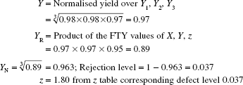
Normalised yield (YN)
Suppose there are x processes, the rolled yield (YR) is the product of the FTY values of each of the x processes. Normalised yield denoted by YN is a value of yield that is same for each process such that
(YN)x = YR
Therefore, normalised yield YN for a set of x processes is
Illustration 16
There are three processes X, Y and z. Find the FTY of Y, YN and YR of set of processes X, Y and z. Find the value of z over all the processes.

where
Annexure 12A deals with a number of exercises on the calculations related to Six Sigma technique.
Process capability analysis (PCA)
Process capability is fundamentally a measure of the minimum defect/error rate in a process or the maximum of its defect/error free output. ‘z’ the Sigma-value of a process, explained and illustrated in this chapter, plays a key role in PCA as under:
- The ideal value of ‘z’ for a process irrespective of its nature and type is 4.5 and this value corresponds to the near-zero defect level of 3.4 ppm. Attaining this level is termed as ‘Six Sigma’ level.
- As the value of z deviates from 4.5 on its lower side, the defect rate increases.
- Defect means a situation that is not as per requirement and the requirement can be an attribute as well as a measurable characteristic. Therefore, the defect rate corresponding to the process includes non-conformance as per attribute as well as measurable characteristics.
- As a first step, assess the z value of the process. In case the value of z is below 4.5, examine the defects and their type. In case the defects are due to lack of conformance to measurable characteristics, then the need arises to assess the ability of the process to meet the required specifications through the technique of X-bar and R chart explained in Chapter 19.
- Improve the capability through (i) various measures explained in the seven scanning tools of Chapters 5 to 11; (ii) elimination of process delays explained in Chapter 13 and (iii) special investigation tools explained in Chapters 18, 19 and 25. All these measures help to improve the capability through defect prevention as well as reduction in variation.
In the opinion of the authors, PCA in most of the Statistical Process Control (SPC) programmes is not addressed as stated above and it is confined only to use of X-bar and R chart which is restrictive, inadequate besides being misleading as it ignores attributes regarding ability. This few decades old deficiency needs to be set right.
Conclusion
The authors wish to conclude this chapter with their observation that the tool of Six Sigma has not made as much progress as other tools of quality control in field of Continual Improvement (CIP). This is due to three factors—elitism attached to Six Sigma; looking upon Six Sigma as a distinctly different entity from CIP with great emphasis on techniques; focusing on jargonising instead of giving attention on instilling the spirit of enquiry supported by creativity and innovation. These aspects which are highlighted succinctly in Chapters 14, 23 and 27 need to be addressed by the quality fraternity and thus accelerate the Six Sigma propagation.
Annexure 12A
Exercises on Six Sigma calculations
Exercise 1
FTY values in four processes are as follows:
Find YR, YN, defect level and z, overall the processes.


z value from table corresponding to a defect level of 0.1577 of a process is 1.01.
Exercise 2
For a production of 10,000 and YR of 96% and having four opportunities, find the number of defects, DPU and DPO.
YR = 0.96, defect rate = 1–0.96 = 0.04
Number of defects in an output of 10,000 = 10,000 × 0.04 = 400

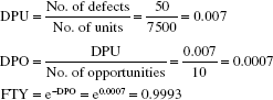
Exercise 3
Fifty defects were found in 7500 units. Ten different types of defects could occur. Find DPU, DPO and FTY at opportunity level.
Exercise 4
Obtain the z and FTY values for eight operations of a seat belt buckle assembly from the data in Table 12.17.
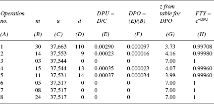
TABLE 12.17 Data for Obtaining z and FTY
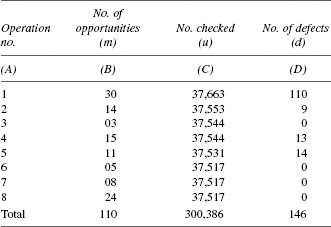
TABLE 12.18 Calculation for Obtaining z and FTY
Exercise 5
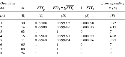
In the Exercise 5, obtain z values on the basis of FTY0 using the FTY results obtained in Exercise 4 presented in Table 12.18.
TABLE 12.19 Calculation of z Values Based on FTY
Exercise 6
Obtain DPU, DPO and z values for the data on defects in 10 drawings summarised in Table 12.20.
TABLE 12.20 Details of Calculations for Obtaining z Value
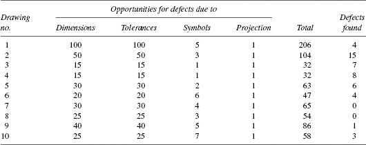
Note: Total no. of units = 10; total no. of opportunities = 747; total no. of defects = 48.

z value corresponding to DPO = 0.064257 is 1.52.
Exercise 7
There are six boxes each having 10 cups. Three cups are found to have a scratch mark. What is the probability that a box does not have a scratch mark.

Exercise 8
Obtain YR, YN and z values from the following data in Table 12.21 related to each process as well as process chain of five processes.
TABLE 12.21 Data for Obtaining YR, YN and z Values

Individual process
The illustration in Table 12.22 explains the method of assessing the z value and FTY of individual processes as well as that of the entire chain of processes.
TABLE 12.22 Details of Calculations for z, and FTY of Individual Processes

*Obtained from the ‘z’ table.
Process chain

z value corresponding to 0.0671 is 1.50.
Note: For use of z table, it has already been mentioned that DPO has to be used to get the Sigma value of the process.
Exercise 9
For the following data derived from Exercise 8, obtain the value of FTY at opportunity level for each process as well as for the overall process; also obtain z values for both. Verify that the z values tally in both Exercises 8 and 9.
TABLE 12.23 Data on m and FTY
| Operation no. | m | FTY of process as e-DPU |
|---|---|---|
| 1 2 3 4 5 |
7 5 10 13 8 |
0.96079 0.88958 0.87985 0.91943 0.86070 |
FTY at opportunity level is given in Table 12.24.
TABLE 12.24 Calculation of z Value of Individual Processes

FTY at opportunity level over all the five processes
z value corresponding to the defect level is 1.51.
z values tally with those of Exercise 8.