You want to create musical notes corresponding to traditional musical notation.

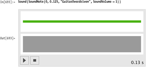
The Mathematica function SoundNote represents a musical sound. SoundNote uses either a numerical convention, for which middle C is represented as zero, or it accepts strings like "C", "C3", or "Aflat4", where "A0" represents the lowest note on a piano keyboard.

SoundNote assumes you want to play a piano sound, for exactly one second, at a medium volume. You can override these presets. Here’s a loud (Soundvolume→1), short (0.125 second), guitar blast ("GuitarOverdriven").

You want to create a sequence of notes, like a scale or single-note melody.

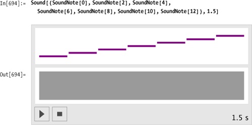
Sound can accept a list of notes, which it will play sequentially. Here is a whole-tone scale specified to take exactly 1.5 seconds to play in its entirety.

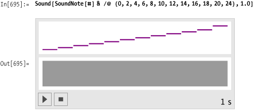
Here’s an alternative syntax using Map (/@), which requires less typing and collects the note specifications into a list.

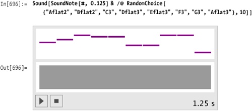
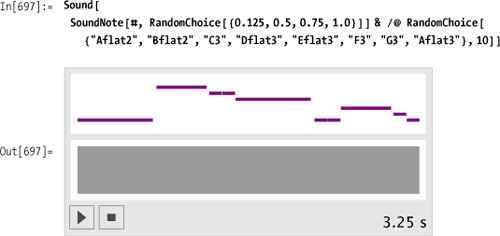
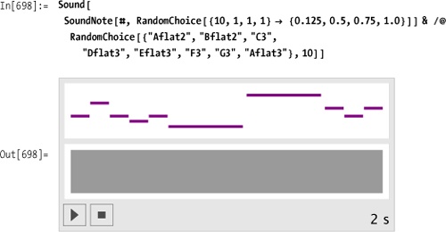
Here’s a randomly generated melody composed of notes from an Ab major scale. The duration of each note is specified as 0.125 second. The duration specification, now a parameter of SoundNote rather than an overall specification of the entire melody as in the previous examples, sets the stage for the next example.

You need to specify a melody for which the notes have different rhythm values.

Replace the 0.125 specification in the previous example with other values. Since you’re generating a random melody, why not generate random durations?

Here, the weighting feature of RandomChoice is used to guarantee a preponderance of short notes.

You would like to add some phrasing to your melody by controlling the volume.

Unlike duration, which is specified as a parameter to SoundNote, you control the volume with an option setting. Pulling everything together from the examples above and adding a randomized volume yields this funky guitar pattern. Anyone for a cup of Maxwell House coffee?

You want to move beyond simple sequences of single notes to chord patterns.

To make a chord, give SoundNote a list of notes. For example, you can specify the C major triad using the pitches C, E, and G specified as a list of numbers {0,4,7}. Don’t confuse making chords by giving SoundNote a list of notes with making melodies by giving Sound a list of SoundNotes.

You want to make a chord progression.

This is the same as making melodies. Spell out the chords in your chord progression as lists inside a list. Feed them into SoundNote using Map.

Here’s a popular pop song progression.

You want to specify a chord progression using traditional notation. For example, you would like to write something like:

In[703]:= myProg = "C A7 d-7 F/G C";

or, using roman numerals as is common in jazz notation,

In[704]:= myJazzProgression = "<Eb> I vi-9 II7/#9b13 ii-9 V7sus I";

Mathematica can deftly handle this task with its String manipulation routines and its pattern recognition functions. First, decide which chord symbols will be allowed. Here’s a list of jazz chords: Maj7/9, Majadd9, add9, Maj7#11, Maj7/13, Maj7/#5, Maj7, Maj, -7b5, -7, -9, -11, min, 7/b913, 7/#9b13, 7/b9b13, 7/b9#11, 7/b5, 7/b9, 7/#9,7/#11,7/13,7,7/9, 7sus, and sus.

The rules below turn the chord names into the appropriate scale degree numbers in the key of C. Later, as a second step, you’ll transpose these voicings to other keys.

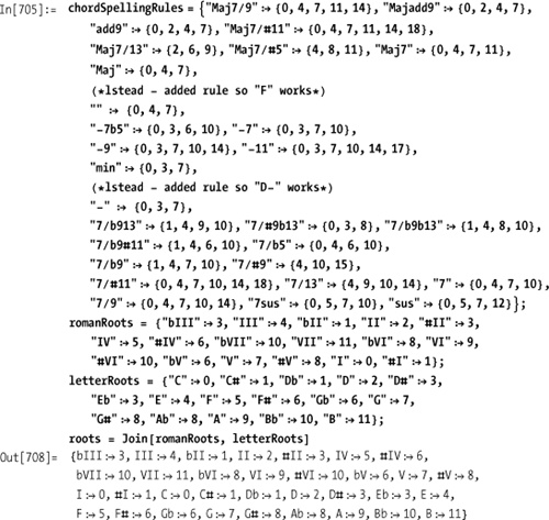
Make a table by concatenating together each possible root and type. Then /. can be used to decode chord.

Now create a function for converting the chord string into a progression representation.

And a function to play the progression.

In[713]:= playProgression[progression[k_, csyms_, kn_, chords_]]:=
           Sound[SoundNote[#, 1] & /@chords, 5]

Let’s test it on a jazz progression.

Let’s add some rhythm and volume.

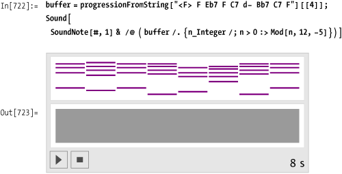
There’s a very unsatisfying feature to the result: the chords jump around in an unmusical way. A piano player would typically invert the chords to keep the voicings centered around middle C. So for example, when playing a CMaj7 chord, which is defined as {0,4,7,11} or {"C3","E3","G3","B3"}, a piano player might drop the tap two notes down an octave and play {-5,-1,0,4} or {"G2","B2","C3","E3"}. You can use Mathematica’s Mod function to achieve the same result. Here the notes greater than 6 {"F#3"} are transposed down an octave simply by subtracting 12 from them.

In[719]:= buffer
Out[719]= {{-21, 3, 7, 10}, {-12, 12, 15, 19, 22, 26}, {-19, 5, 8, 13},
           {-19, 5, 8, 12, 15, 19}, {-14, 10, 15, 17, 20}, {-21, 3, 7, 10}}

Currently in the buffer, the nonbass notes are all positive, so this rule, which uses /; n>0 as a condition, leaves the (negative) bass notes untouched while processing the rest of the voicing.

Here’s another progression showing all the steps in one place.

You want to make percussion sounds.

Mathematica has implemented 60 percussion instruments as specified in the General MIDI (musical instrument digital interface) specification.

Here the percussion instruments are listed in alphabetical order. Some of the names are not obvious. For example, there is no triangle or conga, instead there’s "MuteTriangle", "OpenTriangle", "HighCongaMute", "HighCongaOpen", and "LowConga".

In [724]:= allPerc = {"BassDrum", "BassDrum2", "BellTree", "cabasa", "Castanets",
               "ChineseCymbal", "Clap", "Claves", "Cowbell", "CrashCymbal",
               "CrashCymba12", "ElectricSnare", "GuiroLong", "Guiroshort", "HighAgogo",
               "HighBongo", "HighCongaMute", "HighCongaOpen", "HighFloorTom",
               "HighTimbale", "HighTom", "HighWoodblock", "HiHatClosed", "HiHatOpen",
               "HiHatPedal", "JingleBell", "LowAgogo", "LowBongo", "LowConga",
               "LowFloorTom", "LowTimbale", "LowTom", "LowWoodblock", "Maracas",
               "MetronomeBell", "MetronomeClick", "MidTom", "MidTom2", "MuteCuica",
               "MuteSurdo", "MuteTriangle", "Opencuica", "Opensurdo", "OpenTriangle",
               "RideBell", "RideCymbal", "RideCymba12", "ScratchPull", "ScratchPush",
               "Shaker", "SideStick", "Slap", "Snare", "SplashCymbal", "SquareClick",
               "Sticks", "Tambourine", "Vibraslap", "WhistleLong", "WhistleShort"};

Here’s what each instrument sounds like. The instrument name is fed into SoundNote where, more typically, the note specification should be. In fact, in the Standard MIDI specification, each percussion instrument is represented as a single pitch in a "drum" patch. So for example, "BassDrum" is CO, "BassDrum2" is C#O, "Snare" is DO, and so on. Therefore, it makes sense for Mathematica to treat these instruments as notes, not as "instruments" as was done above for "Piano", "GuitarMuted", and "GuitarOverDriven".

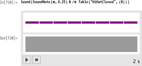
Here’s a measure’s worth of closed hi-hat:

And here’s something with a little more pizzazz. Both the choice of instrument and volume are randomized.

You want to create a drum kit groove for a pop song using kick, snare, and hi-hat.

This task is the percussion equivalent of making chords, because on certain beats all three instruments could be playing, on other beats only one instrument or possibly none. Here’s the previous hi-hat pattern, played at a slower tempo.

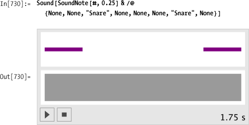
Here’s a kick drum pattern. Use None as a rest indication.

Here’s the snare drum backbeat. The display omits the leading rests, so the picture is a little misleading. As soon as we integrate this with the hi-hat and kick drum, everything will look correct.

Each list has exactly eight elements, so we can use Transpose to interlace the elements.

In[731]:=  groove = Transpose[{Table["HiHatClosed", {8}],
               {"BassDrum", None, None, "BassDrum", "BassDrum", None, None, None},
               {None, None, "Snare", None, None, None, "Snare", None}}]
Out[731]=  {{HiHatClosed, BassDrum, None}, {HiHatClosed, None, None},
            {HiHatClosed, None, Snare}, {HiHatClosed, BassDrum, None},
            {HiHatClosed, BassDrum, None}, {HiHatClosed, None, None},
            {HiHatClosed, None, Snare}, {HiHatClosed, None, None}}

An entire tune can now be made by repeating this one-measure groove as many times as desired.

Getting the curly braces just right in Mathematica’s syntax can be a little frustrating. Without Flatten in the example above, the SoundNote function is confused by the List-within-List results of the Table function. Consequently, you get no output.

In[734]:=  Sound[SoundNote[#, 0.25] &/@ Table[groove, {4}]]

Out[734]=  Sound[
            {SoundNote[{{"HiHatClosed", "BassDrum", None}, {"HiHatClosed", None, None},
               {"HiHatClosed", None, "Snare"}, {"HiHatClosed", "BassDrum", None},
               {"HiHatClosed", "BassDrum", None}, {"HiHatClosed", None, None},
               {"HiHatClosed", None, "Snare"}, {"HiHatClosed", None, None}}, 0.25`],
             SoundNote[{{"HiHatClosed", "BassDrum", None}, {"HiHatClosed", None, None},
               {"HiHatClosed", None, "Snare"}, {"HiHatClosed", "BassDrum", None},
               {"HiHatClosed", "BassDrum", None}, {"HiHatClosed", None, None},
               {"HiHatClosed", None, "Snare"}, {"HiHatClosed", None, None}}, 0.25'],

           SoundNote[{{"HiHatClosed", "BassDrum", None}, {"HiHatClosed", None, None},
               {"HiHatClosed", None, "Snare"}, {"HiHatClosed", "BassDrum", None},
               {"HiHatClosed", "BassDrum", None}, {"HiHatClosed", None, None},
               {"HiHatClosed", None, "Snare"}, {"HiHatClosed", None, None}}, 0.25`],
             SoundNote[{{"HiHatClosed", "BassDrum", None}, {"HiHatClosed", None, None},
               {"HiHatClosed", None, "Snare"}, {"HiHatClosed", "BassDrum", None},
               {"HiHatClosed", "BassDrum", None}, {"HiHatClosed", None, None},
               {"HiHatClosed", None, "Snare"}, {"HiHatClosed", None, None}}, 0.25`]}]

Furthermore, with a simple Flatten wrapped around the Table function, each hit is treated individually; we lose the chordal quality of the drums hitting simultaneously. Go back and notice that the correct idea is to remove just one layer of braces by using Flatten [ ... , 1 ].

You want to save your Mathematica expression as a standard MIDI file.

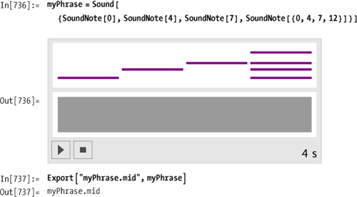
Mathematica can export any expression composed of Sound and SoundNote expressions as a standard MIDI file. The rub, however, is that Mathematica does not import MIDI files. So let’s create some utilities that at the very least let you look at the guts of standard MIDI files.

Here’s a simple phrase that gets exported as the file myPhrase.mid.

You want to listen to the waveform generated by a mathematical function.

If you know how to plot a function in Mathematica:

You can play a function. Play uses the same syntax as Plot. However, you don’t want to listen to 1/1000th of a second, which is what was plotted above, so specify something like {t, 0, 1}.

Here are other crazy-sounding functions.

You want to add tremolo.

"Tremolo" is the musical term for amplitude modulation. Here a 20 Hz signal modifies the amplitude of a 1,000 Hz signal.

And here, a 5 Hz signal modifies a 1,000 Hz signal.

You want to add vibrato.

Vibrato is frequency modulation. Notice that the sine wave alternates between regions of compression and expansion.

Here the parameters are adjusted for listening.

Why not put the two modulations together: tremolo and vibrato?

You want to apply an envelope to your signal.

The Mathematica function Piecewise is the perfect tool for creating an envelope. Here is the popular attack-decay-sustain-release (ADSR) envelope.

Sine waves are typically represented as amplitude * sine (ωt). You can simply substitute the entire Piecewise[] envelope for amplitude.

Listen!

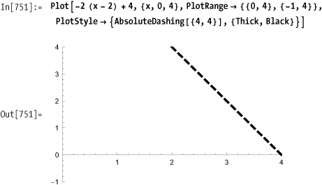
Calculating the envelope functions for the four regions is not as hard as you might expect. Perhaps you remember the equation for a straight line: y = m x + b, where m is the slope of the line and b is the y-intercept. Here is a line with a slope of -2 that intercepts the y-axis at y = 4, so its equation is y = -2x + 4.

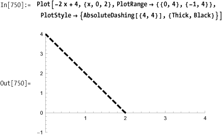
If this were the function for the second portion of the envelope, the decay portion, you would need to shift this line to the right. You can shift the line to the right simply by replacing x with (x - displacement). In general, the template for creating the equations for the Piecewise functions will be: y = m (x - displacement) + initial value of segment. Notice that what was at first the y-intercept is now the "initial value of the segment." The line here is shifted two units to the right, and the new equation is y = -2 (x - 2) + 4. If we simplify the right side, the equation becomes y = -2x + 8. This line has the same -2 slope but would intercept the y-axis at y = 8 if we were to extend the line to the left.

You want to explore different partitions of the musical scale and alternate instrument tunings.

Modern Western music uses tempered tuning, which is a slight compromise to the vibrations of the natural world, or at least the perfection of the natural world as the Greeks described it 3,000 years ago. The ancient Greeks (and even earlier, the Babylonians) noticed that when objects vibrate in simple, integer ratios to each other, the resulting sound is pleasant. The simple ratio of 2:1 is so pleasant that we perceive it as an equivalence. When two notes vibrate in a ratio of 2:1, we say they have the same pitch but are in different octaves. The history of music has been the history of partitioning the octave.

The first obvious division of the octave is created by the next simplest ratio, a 3:1 ratio. Consider the following schematic of a vibrating string. The only requirement on the string is that its endpoints remain fixed. The string can vibrate in many different modes, as shown in the first column. Each mode has a characteristic number of still points, called "nodes," that appear symmetrically along the length of the string. Each mode also has a characteristic rate of vibration, which is a simple integer multiple to the lowest fundamental frequency. Notice that three out of the first four harmonics are octave equivalences. The third harmonic, situated between the second and fourth harmonics, has a ratio of 3:2 to the second harmonic and 3:4 to the fourth. These were the kinds of simple ratios that appealed to the Greeks.

The following keyboard shows how a successive application of the 3:2 ratio can be used to build the entire chromatic scale. After 12 applications of this 3:2 ratio, every note of the modern chromatic scale has been visited once and we are returned to starting pitch—sort of!

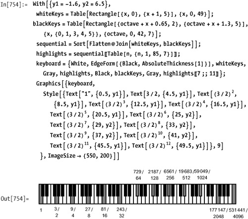
There’s a problem: (3/2)¹² represents the C seven octaves above the starting C and should equal a C with a frequency ratio of 2⁷ = 128, but (3/2)¹² equals 129.75. The equal temperament solution to this problem is to distribute this discrepancy equally over all the intervals. In other words, in equal temperament, every interval is made slightly, and equally, "out of tune." Johann Sebastian Bach composed a series of keyboard pieces in 1722 called "The Well-Tempered Clavier" to demonstrate that this compromise was basically imperceptible and had no negative impact on the beauty of the music.

Mathematically, equal temperament means that the frequency of each pitch should have the same ratio to its immediate lower neighbor’s frequency. Call this ratio α. Then it must be the case that if a chromatic scale, which contains 12 pitches, takes you from some frequency to twice that frequency, then α¹²= 2. So the ratio of a semitone in equal temperament is 1.0596.

However, now that we have the octave in perfect shape, every other interval is slightly "wrong"—or at least wrong according to the manner in which the Greeks were trying to make their intervals. So for example, a Pythagorean fifth, which is 3/2 = 1.5, is slightly flat in equal temperament (the musical interval of a fifth is composed of seven half-steps).

In[756]:= α7
Out[756]= 1.498317

In[757]:= 1.498307
Out[757]= 1.49831

Now that we’ve gone through the basics of tuning, how do you use Mathematica to explore alternate tunings?

As explained above, tuning instruments in the modern Western world is based on dividing the octave into 12 equal segments. If the ratio of the semitone C to C# is called α, then the ratio of the octave from C3 to C4 is α¹² and should equal 2.0. Therefore you can calculate α to be the 12th root of 2.0.

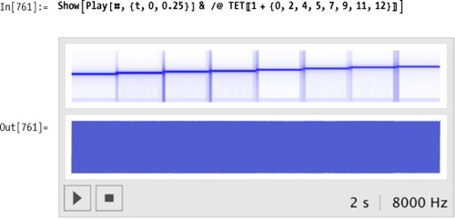
Here’s the equal-tempered chromatic scale, sometimes referred to as 12-TET (twelvetone equal temperament):

In[759]:= TET = Table[Sin [440.0 * αn * 2 π * t], {n, 0, 12}]
Out[759]= {Sin[2764.6 t], Sin[2928.99 t], Sin[3103.16 t],
           Sin[3287.68 t], Sin[3483.18 t], Sin[3690.3 t],
           Sin[3909.74 t], Sin[4142.22 t], Sin[4388.53 t],
           Sin[4649.49 t], Sin[4925.96 t], Sin[5218.87 t], Sin[5529.2 t]}

 Out[96]= {Sin[2764.6 t], Sin[2928.99 t], Sin[3103.16 t],
           Sin[3287.68 t], Sin[3483.18 t], Sin[3690.3 t],
           Sin[3909.74 t], Sin[4142.22 t], Sin[4388.53 t],
           Sin[4649.49 t], Sin[4925.96 t], Sin[5218.87 t], Sin[5529.2 t]}

          {Sin[2764.6 t], Sin[2928.99 t], Sin[3103.16 t],
           Sin[3287.68 t], Sin[3483.18 t], Sin[3690.3 t],
           Sin[3909.74 t], Sin[4142.22 t], Sin[4388.53 t],
           Sin[4649.49 t], Sin[4925.96 t], Sin[5218.87 t], Sin[5529.2 t]}

The equal-tempered major scale is

You want to import a digital sound file, for example, a WAV or AIFF file.

Mathematica imports many standard file formats. Both AIFF and WAV are in the list.

In[762]:= $ImportFormats
Out[762]= {3DS, ACO, AIFF, ApacheLog, AU, AVI, Base64, Binary, Bit, BMP, Byte, BYU,
           BZIP2, CDED, CDF, Character16, Character8, Complex128, Complex256,
           Complex64, CSV, CUR, DBF, DICOM, DIF, Directory, DXF, EDF, ExpressionML,
           FASTA, FITS, FLAC, GenBank, GeoTIFF, GIF, Graph6, GTOPO30, GZIP,
           HarwellBoeing, HDF, HDF5, HTML, ICO, Integer128, Integer16, Integer24,
           Integer32, Integer64, Integer8, JPEG, JPEG2000, JVX, LaTeX, List, LWO,
           MAT, MathML, MBOX, MDB, MGF, MMCIF, MOL, MOL2, MPS, MTP, MTX, MX, NB,
           NetCDF, NOFF, OBJ, ODS, OFF, Package, PBM, PCX, PDB, PDF, PGM, PLY, PNG,
           PNM, PPM, PXR, QuickTime, RawBitmap, Real128, Real32, Real64, RIB,
           RSS, RTF, SCT, SDF, SDTS, SDTSDEM, SHP, SMILES, SND, SP3, Sparse6, STL,
           String, SXC, Table, TAR, TerminatedString, Text, TGA, TIFF, TIGER,
           TSV, UnsignedInteger128, UnsignedInteger16, UnsignedInteger24,
           UnsignedInteger32, UnsignedInteger64, UnsignedInteger8, USGSDEM, UUE,
           VCF, WAV, Wave64, WDX, XBM, XHTML, XHTMLMathML, XLS, XML, XPORT, XYZ, ZIP}

Using the "Data" specification will save you the aggravation of decoding the syntax of the imported data. Don’t forget the semicolon, which prevents Mathematica from listing all the sample points. The easiest way to access a file is to type Import[ ], place your cursor between the empty brackets, choose File... from the Insert Menu, navigate in the dialog box to the file you want to open.

In[763]:= file = FileNameJoin [{NotebookDirectory [], "..", "data", "JCK_01.aif"}];
          data = Flatten@Import[file, "Data"];

You’ll need to know the sample rate and whether this file is a mono or stereo, so do a second Import on the same file but specify "Options".

If you simply wanted to play the file, specify "Sound" as the second parameter.

In[766]:=  snd = Import[file, "Sound"];

This returns a Sound object.

In[767]:=  snd // Head
Out[767]=  Sound

And can be played like so:

Sound files can be huge, and as such, become difficult to work with.

In[769]:=  Length [data]
Out[769]=  1396853

Here’s a quick way to get an overview of a sound file. Mathematica is being asked to display every thousandth sample point. You can easily see there are a handful of bursts of energy.

Focus on the three wavelets between 900,000 and 1,300,000.

"Yes we can; yes we can; yes we can!"

You want to do a Fourier analysis on a sound file. Fourier analysis is a means of investigating the energy in a signal. Specifically, Fourier analysis will report on the energy spectrum of a signal versus frequency. The mathematics behind Fourier analysis is quite sophisticated, but armed with just a few principles, you can put Mathematica’s Fourier tools to work for you.

Typically you’ll start with a digitized signal. The sampling rate will determine the highest frequency that can be investigated. This highest frequency is called the Nyquist frequency and is always exactly one half the sampling rate. For this "Yes we

can!" sample, which was digitized at 48 KHz, the highest frequency is 24 KHz. (It’s not coincidental that this frequency is slightly greater than the limits of human hearing.) Notice the plot is symmetric about the Nyquist frequency.

The number of sample points used in any analysis is also critical. Here exactly one second of audio, that is, 48,000 sample points, is being analyzed. The 48,000 points from the time domain yield 48,000 points in the frequency domain, but as you can see, the right side of the plot, between points 24,000 and 48,000, is just a mirror duplication of the points between 0 and 24,000. This is an artifact of the underlying mathematics, and there is no additional information in this half of the plot.

Since this is speech, you can focus on the first 2,000 points, which correspond to frequencies 0 to 2,000 Hz. Later you’ll see that 2,000 points of a Fourier analysis doesn’t always mean frequencies 0 through 2,000 Hz. It does in this case because you started with 48,000 sample points in the time domain that equals the sampling rate and created a one-to-one relationship between data points and frequencies in the frequency domain. You can see that this speaker has four significant frequency resonances to his voice at approximately 150 Hz, 300 Hz, 490 Hz, and 700 Hz. These resonances are known as formants. Notice, the Ticks option customized the labeling of the x-axis.

Typically, when analyzing voice, one second is too long of a sample. Just think how many syllables you utter in one second of normal speech. A much more appropriate length would be 1/10 or 1/20 or even 1/30 of a second. You can easily identify various phonemes of "yes we can" in the plot below: the "yeh" and "sss" of the "yes," the singular vowel sound of "we," and the hard "c" and "an" of "can."

Here’s the "we," which is very homogeneous.

You’re now looking at 9,600 sample points (9,600/48,000 = 1/5 sec) in the time domain, so each point in the frequency domain represents 48,000/9,600 = 5 Hz. There’s a direct trade-off between using as few sample points as possible to narrow the analysis to a single phoneme, versus sampling enough points to ascertain a desired precision in the frequency domain.

Here, half as many points (4,800) sampled from the same region focuses our analysis in the time domain, but each sample point now represents 10 Hz. Perhaps we’re losing some detail in the 150-200 Hz range, as well as the 300-350 Hz range?

You want a Fourier analysis over time.

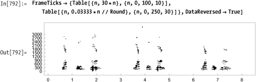
You can partition the data into 1/30 of a second slices and do an analysis on each slice. Each sample point in the frequency domain will be 30 Hz, which is "wider" than the previous examples, but the precision in the time domain will more than make up for it.

Take just the lowest 100 frequency bands, frequencies 0-3,000 Hz.

With Mathematica’s Graphics3D primitives, you can make this waterfall-style chart, where time is left to right across the front, and frequency is front to back.

ListLinePlot accomplishes the same thing but interpolates the individual lines into surfaces.

Now that you’ve seen the previous 3D displays, perhaps these contour plots will make immediate sense to you. These are bird’s-eye views of the 3D plots. You can really finesse these plots to bring out the details. Look at the color versions provided in the online version of this book.

Tweaking the Contours and ContourShading options prevent the white-outs in the peak regions.

A Spectrograph

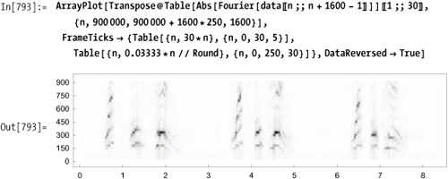
ArrayPlot is another perfect tool to display the results. ArrayPlot will automatically scale the results such that the greater the energy content in the frequency domain, the darker the plot. Frequency runs across the page, as shown previously in 9.17 Analyzing Digital Sound Files, whereas the individual slices run down the page.

You can improve on ArrayPlot's formatting. Convention wants time to run left to right across the page and frequency to run bottom to top. Transpose will reverse the axes, but you’ll also need DataReversed→True to make time run left to right.

You could set a threshold and display in black and white.

Or, you could zoom in and look more closely at the lower frequencies.