You can’t understand why you are getting a particular result but suspect it is due to a false assumption or bug in an intermediate calculation whose value is not visible.

Injecting a strategically placed Print statement can often be the quickest path to debugging a small piece of code. Suppose you forgot or did not know Mathematica’s convention for choosing branches in the Power[x,y] function (it prefers the principal value of e^{y log (x)}).

In[1]:= x =-1;
        y = Power [x, 1/3];
        If[ y == -1, "expected", "not expected"]
Out[3]= not expected

Here is the same code with a Print inserted so the value of y can be inspected. You will often want to force numerical conversion using N[] when inserting Print; otherwise you would get the symbolic value (in this case -1^(1/3)), which is quite unhelpful.

Anyone who has spent even a day programming has come across this obvious debugging technique, so it may seem hardly worth a whole recipe, but please read on. Sometimes, injecting Print into code is very inconvenient, especially if you code in tight function style with few intermediate values appearing in variables. The problem is that you can’t inject Print into functional code because Print does not return a value. Consider if the code for the value y did not exist because it was in-lined.

In[7]:= x = -1;
        If[ Power[x, 1/3] == -1, "expected", "not expected"]
Out[8]= not expected

You can’t wrap the call to Power in a Print because it would change the behavior of the expression, which is not what you want to do when you are already contending with bugs. For these situations, it is handy to whip up a functional version of Print, which I call fPrint. This saves you the trouble of introducing temporary variables for purposes of debugging, thus leaving less mess to clean up after you have diagnosed the problem.

A possible problem that can lead to lost or gray hairs when debugging with Print is when it seems to print nothing. This can take you down the road to hell by misleading you into thinking your code must be taking a different branch. For example, it is easy to miss the empty print cell created by executing this code.

This is not as contrived as it may seem: there are bugs that arise from failure to consider the fact that a sequence might be null, for example, when you use Apply (@@) on an empty list.

Here an error was generated, and the output was "something completely different" because the expression in the If was neither True nor False. Pretend it was not immediately obvious to you what was going on (after all, you clearly see that you called Total with one argument x). You decide to use Print to get to the bottom of it. Notice that introducing Print into this code requires the whole thing to be wrapped in parentheses (another common debugging pitfall).

If you were confused before, you are now totally befuddled! Here is where your own little functional fPrint can help, but you need to tweak it slightly to expose two common ghosts you might encounter in the wild.

In[18]:= Clear[fPrint];
         fPrint[] := (Print["NullSequence!!"]; Unevaluated[Sequence[]])
         fPrint[""] := (Print["NullString!!"]; "")
         fPrint[x__] := (Print[x]; x)

Now the problem is revealed, and you also side-stepped the parenthesis mistake.

There are other output functions (PrintTemporary, CellPrint, and MessageDialog) that may be useful in certain debugging situations. See the documentation for these functions. I use PrintTemporary as part of the solution in 19.5 Creating a Poor Man’s Mathematica Debugger.

You have a function that is invoked thousands of times, but only a few of the calls produce an unexpected result, and it is difficult to determine which invocations are causing the problem. Print is a poor choice because of the unreasonable amount of data that may get printed before you identify the issue.

Use the Reap-Sow combination discussed in 2.10 Incremental Construction of Lists to capture the data so you can analyze it using pattern matching or plotting. For example, imagine you have a function called func that is returning unexpected negative values and you are trying to understand the arguments that lead up to negative results. Here I use a contrived function for sake of the example. You can write a little wrapper around the function like so.

In[24]:= func[a_, b_, c_, d_] := If [a + 16 < b + c, 1 - d, b + c]
         funcWrapper[args__] :=
          Module[{r}, r = func[args] ; If [r < 0, Sow [{args}]]; r]
         {result, {problem}} =
           Reap[Table[funcWrapper[a, b, c, d], {a, 10}, {b, 10}, {c, 10}, {d, 10}]];

You can now see that there are 90 sets of arguments that caused the negative condition. Furthermore, you have the exact problematic values captured in a variable and can use the values to debug the function using techniques presented in other recipes in this chapter.

In[27]:= Length[problem]
Out[27]= 90

Invoking the function on these problematic arguments is a cinch using @@@.

In[28]:= func @@@ problem
Out[28]= {-1, -2, -3, -4, -5, -6, -7, -8, -9, -1, -2, -3, -4, -5, -6, -7, -8, -9,
          -1, -2, -3, -4, -5, -6, -7, -8, -9, -1, -2, -3, -4, -5, -6, -7, -8, -9,
          -1, -2, -3, -4, -5, -6, -7, -8, -9, -1, -2, -3, -4, -5, -6, -7, -8, -9,
          -1, -2, -3, -4, -5, -6, -7, -8, -9, -1, -2, -3, -4, -5, -6, -7, -8, -9,
          -1, -2, -3, -4, -5, -6, -7, -8, -9, -1, -2, -3, -4, -5, -6, -7, -8, -9}

Reap-Sow are a powerful debugging tool because they can direct debug data into an arbitrary number of channels. By channel, I refer to the capability of Sow to specify a tag as a second argument such that all instances of Sow with that tag collect data into a distinct list. For example, imagine you want to detect when func returns zero but want to segregate those arguments from the arguments that cause negative results.

In[29]:= funcWrapper[args__] := Module[{r}, r = func[args] ;
           Which[r < 0, Sow[{args}, negative], r == 0, Sow[{args}, zero], True, 0]; r]

In[30]:= {result, {{n}, {z}}} = Reap[Table[funcWrapper[a, b, c, d],
              {a, 10}, {b, 10}, {c, 10}, {d, 10}], {negative, zero}];

Now you can use these values as separate test sets to understand these distinct behaviors.

In[31]:= func @@@ n
Out[31]= {-1, -2, -3, -4, -5, -6, -7, -8, -9, -1, -2, -3, -4, -5, -6, -7, -8, -9,
          -1, -2, -3, -4, -5, -6, -7, -8, -9, -1, -2, -3, -4, -5, -6, -7, -8, -9,
          -1, -2, -3, -4, -5, -6, -7, -8, -9, -1, -2, -3, -4, -5, -6, -7, -8, -9,
          -1, -2, -3, -4, -5, -6, -7, -8, -9, -1, -2, -3, -4, -5, -6, -7, -8, -9,
          -1, -2, -3, -4, -5, -6, -7, -8, -9, -1, -2, -3, -4, -5, -6, -7, -8, -9}

In[32]:= func @@@ z
Out[32]= {0,0,0,0,0,0,0,0,0,0}

19.6 Debugging Built-In Functions with Evaluation and Step Monitors shows another common application of Reap-Sow in the debugging of built-in numerical algorithms or plotting functions.

19.3 Stack Tracing to Debug Recursive Functions shows how to use Reap-Sow to take Stack snapshots.

You have a recursive function that is unexpectedly violating $RecursionLimit and generating an error. Alternatively, you have a complex function with many function calls and you want to understand the sequence of calls that leads up to an error condition or erroneous value.

Use Stack[] to output a stack trace. Here I use Ackermann’s function to illustrate the use of Stack because it will easily violate any sane recursion limit. Further, I create a function that will detect stack overflow before it happens and Throw the stack to caller. Specifically, I throw those expressions on the stack that match the function of interest by using Stack[A].

In[33]:= debugStack[] :=
           If[Length[Stack[]] + 1 ≥ $RecursionLimit, Throw[Stack[A]]];
         A[0, n_]  := n + 1
         A[m_, 0]  := (debugStack[]; A[m - 1, 1])
         A[m_, n_] := (debugStack[]; A[m - 1, A[m, n -1]])

In[37]:= Catch[Block[{$RecursionLimit = 30}, A[4, 1]]]
Out[37]= {A[4 - 1,A[4, 1 - 1]],A[2 - 1,A[2, 5 - 1]],
          A[2 - 1,A[2, 4 - 1]],A[1 - 1,A[1, 7 - 1]],
          A[1 - 1,A[1, 6 - 1]],A[1 - 1,A[1, 5 - 1]],A[1 - 1,A[1, 4 - 1]],
          A[1 - 1,A[1, 3 - 1]],A[1 - 1,A[1, 2 - 1]],A[1 - 1,A[1, 1 - 1]]}

If you want to take multiple snapshots of the stack during the progression of the function, regardless whether it overflows or not, you can use Reap-Sow.

 In[38]:= Clear[f]

 In[39]:= f[0] := Module[{}, Sow[Stack[Times]]; 1]
         f[x_] := Module[{}, Sow[Stack[Times]]; x * f [x - 1]]

 In[41]:= Reap[f[3]]
 Out[41]= {6, {{{}, {3f[3 - 1]},
             {3f[3 - 1], 2f[2 - 1]}, {3f[3 - 1], 2f[2 - 1], 1f[1 - 1]}}}}

StackInhibit can be used to keep certain expressions from showing up in the evaluation stack. It can be helpful to insert this function into your code to control the amount of information in the stack. I use this function as part of 19.5 Creating a Poor Man’s Mathematica Debugger.

Trace provides an extremely detailed account of the evaluation of an expression; however, for all but the most trivial expressions, this voluminous detail can be difficult to wade through.

Again, I use the Ackermann function to illustrate the issue, although this problem is not particular to recursive functions. Ackermann is convenient because it creates a large number of nested function calls and intermediate expressions. In addition, I purposefully throw a monkey wrench into this function to simulate a bug: "bug". Real-world bugs don’t come so nicely labeled (if only!) but the point here is that in a real-world debugging situation you are looking for a particular subexpression that looks fishy based on your knowledge of the intended computation.

In[42]:= A[0, n_] := n + 1
         A[m_, 0] := A[m - 1, 1]
         A[m_, 2] := ("bug"; A[m - 1, A[m, 1]])
         A[m_, n_] := A[m - 1, A[m, n - 1]]

If you attempt to trace this buggy Ackermann on even relatively tame inputs, you will quickly generate a lot of output that anyone but the most seasoned Mathematica developer would have trouble deciphering. In essence, what you are seeing is an expansion of the call tree, and thus, the problem is not only the amount of output but the deeply nested structure of the output. You could easily miss the "bug" in this data, and even if you spot it, you might still have trouble understanding what led up to its occurrence.

In[46]:= trace = Trace[A[2, 3]]
Out[46]= {A[2, 3], A[2 - 1, A[2, 3 - 1]], {2 - 1,1},
          {{3 - 1, 2}, A[2, 2], bug; A[2 - 1, A[2, 1]],
           {{2 - 1, 1}, {A[2, 1], A[2 - 1, A[2, 1 - 1]], {2 - 1,1}, {{1 - 1, 0}, A[2, 0],
              A[2 - 1, 1], {2 - 1, 1}, A[1, 1], A[1 - 1, A[1, 1 - 1]], {1 - 1, 0},
              {{1 - 1, 0}, A[1, 0], A[1 - 1, 1], {1 - 1, 0}, A[0, 1], 1 + 1, 2},
              A[0, 2], 2 + 1, 3}, A[1, 3], A[1 - 1, A[1, 3 - 1]],
             {1 - 1, 0}, {{3 - 1, 2}, A[1, 2], bug; A[1 - 1, A[1, 1]],
              {{1 - 1, 0}, {A[1, 1], A[1 - 1, A[1, 1 - 1]], {1 - 1, 0},
                {{1 - 1, 0}, A[1, 0], A[1 - 1, 1], {1 - 1, 0}, A[0, 1], 1 + 1, 2},
                A[0, 2], 2 + 1, 3}, A[0, 3], 3 + 1, 4}, 4}, A[0, 4], 4 + 1, 5}, A[1, 5],
            A[1 - 1, A[1, 5 - 1]], {1 - 1, 0}, {{5 - 1,4}, A[1,4], A[1 - 1, A[1, 4 - 1]],
             {1 - 1, 0}, {{4 - 1, 3}, A[1, 3], A[1 - 1, A[1, 3 - 1]],
              {1 - 1, 0}, {{3 - 1, 2}, A[1, 2], bug; A[1 - 1, A[1, 1]],
               {{1 - 1, 0}, {A[1, 1], A[1 - 1, A[1, 1 - 1]], {1 - 1, 0},
                 {{1 - 1, 0}, A[1, 0], A[1 - 1, 1], {1 - 1, 0}, A[0, 1], 1 + 1, 2},
                 A[0, 2], 2 + 1, 3}, A[0, 3], 3 + 1, 4}, 4}, A[0, 4], 4 + 1, 5},
             A[0, 5], 5 + 1, 6}, A[0, 6], 6 + 1, 7}, 7}, A[1, 7],
          A[1 - 1, A[1,7 - 1]], {1 - 1, 0}, {{7 - 1,6},
           A[1, 6],
           A[1 - 1, A[1, 6 - 1]],
           {1 - 1, 0},
           {{6 - 1, 5}, A[1, 5], A[1 - 1, A[1, 5 - 1]], {1 - 1, 0},
            {{5 - 1,4}, A[1,4], A[1 - 1, A[1,4 - 1]], {1 - 1, 0},
             {{4 - 1, 3}, A[1, 3], A[1 - 1, A[1, 3 - 1]], {1 - 1, 0},
              {{3 - 1, 2}, A[1, 2], bug; A[1 - 1, A[1, 1]], {{1 - 1, 0},
                {A[1, 1], A[1 - 1, A[1, 1 - 1]], {1 - 1, 0}, {{1 - 1, 0}, A[1, 0],
                  A[1 - 1, 1], {1 - 1, 0}, A[0, 1], 1 + 1, 2}, A[0, 2], 2 + 1, 3},
                A[0, 3], 3 + 1, 4}, 4}, A[0, 4], 4 + 1, 5}, A[0, 5], 5 + 1, 6},
           A[0, 6], 6 + 1, 7}, A[0, 7], 7 + 1, 8}, A[0, 8], 8 + 1, 9}

Using Depth, you can see that there are 13 levels in the expression output by Trace (although this is inflated by the existence of HoldForm, as I explain later). In a real-world use of Trace, you could easily encounter output with depth an order of magnitude larger and an overall output several orders of magnitude larger still.

In[47]:= Depth[trace]
Out[47]= 13

To understand this solution, be aware that all the intermediate expressions output by Trace are wrapped in HoldForm to prevent their evaluation (which would of course defeat the purpose of Trace). You can see this by using InputForm. I use Short to suppress repeating the mess of output from above.

   In[48]:=  trace // InputForm // Short
Out[48]//Short=
              {HoldForm[A[2, 3]], HoldForm[A[2
                - 1, A[2, <<1>>]]], <<8>>, HoldForm[9]}

One way to get a handle on the output of Trace is to linearize it so you get a flat structure that presents the sequence of operations as they occur in time. This can be done by using what amounts to a preorder tree traversal.

In[49]:= Clear[traverseTrace, traverseTrace1];
         traverseTrace[x_] := Flatten[Reap[traverseTrace1[x]]]
         traverseTrace1[{}] := Sequence[]
         traverseTrace1[x_List] :=
          (traverseTrace1[First[x]]; traverseTrace1[Rest[x]])
         traverseTrace1[HoldForm[x_]] := Sow[HoldForm[x]]

This still produces as much raw data, but its linear nature makes it easier to visualize and manipulate.

In[54]:= timeSequence = traverseTrace[trace]
Out[54]= {A[2, 3], A[2 - 1, A[2, 3 - 1]], 2 - 1, 1, 3 - 1, 2, A[2, 2], bug;
          A[2 - 1, A[2, 1]], 2 - 1, 1, A[2, 1], A[2 - 1, A[2, 1 - 1]], 2 - 1, 1, 1 - 1,
          0, A[2, 0], A[2 - 1, 1], 2 - 1, 1, A[1, 1], A[1 - 1, A[1, 1 - 1]], 1 - 1,
          0, 1 - 1, 0, A[1, 0], A[1 - 1, 1], 1 - 1, 0, A[0, 1], 1 + 1, 2, A[0, 2],
          2 + 1, 3, A[1, 3], A[1 - 1, A[1, 3 - 1]], 1 - 1, 0, 3 - 1, 2, A[1, 2], bug;
          A[1 - 1, A[1, 1]], 1 - 1, 0, A[1, 1], A[1 - 1, A[1, 1 - 1]], 1 - 1, 0,
          1 - 1, 0, A[1, 0], A[1 - 1, 1], 1 - 1, 0, A[0, 1], 1 + 1, 2, A[0, 2], 2 + 1,
          3, A[0, 3], 3 + 1, 4, 4, A[0,4], 4 + 1, 5, A[1, 5], A[1 - 1, A[1, 5 - 1]],
          1 - 1, 0, 5 - 1, 4, A[1, 4], A[1 - 1, A[1, 4 - 1]], 1 - 1, 0, 4 - 1, 3, A[1,3],
          A[1 - 1, A[1, 3 - 1]], 1 - 1, 0, 3 - 1, 2, A[1, 2], bug; A[1 - 1, A[1, 1]],
          1 - 1, 0, A[1, 1], A[1 - 1, A[1, 1 - 1]], 1 - 1, 0, 1 - 1, 0, A[1, 0],
          A[1 - 1, 1], 1 - 1, 0, A[0, 1], 1 + 1, 2, A[0, 2], 2 + 1, 3, A[0, 3], 3 + 1,
          4, 4, A[0, 4], 4 + 1, 5, A[0, 5], 5 + 1, 6, A[0, 6], 6 + 1, 7, 7, A[1, 7],
          A[1 - 1, A[1, 7 - 1]], 1 - 1, 0, 7 - 1, 6, A[1, 6], A[1 - 1, A[1, 6 - 1]],
          1 - 1, 0, 6 - 1, 5, A[1, 5], A[1 - 1, A[1, 5 - 1]], 1 - 1, 0, 5 - 1, 4, A[1, 4]
          A[1 - 1, A[1, 4 - 1]], 1 - 1, 0, 4 - 1, 3, A[1, 3], A[1 - 1, A[1, 3 - 1]],
          1 - 1, 0, 3 - 1, 2, A[1, 2], bug; A[1 - 1, A[1, 1]], 1 - 1, 0, A[1, 1],
          A[1 - 1, A[1, 1 - 1]], 1 - 1, 0, 1 - 1, 0, A[1, 0], A[1 - 1, 1], 1 - 1, 0,
          A[0, 1], 1 + 1, 2, A[0, 2], 2 + 1, 3, A[0, 3], 3 + 1, 4, 4, A[0, 4], 4 + 1, 5,
          A[0, 5], 5 + 1, 6, A[0, 6], 6 + 1, 7, A[0, 7], 7 + 1, 8, A[0, 8], 8 + 1, 9}

Once you have linearized the output of Trace, you can easily extract segments of the execution history or use patterns to extract specific segments of interest.

   In[55]:=  timeSequence[[5 ;; 18]] // InputForm
Out[55]//InputForm=
             {HoldForm[3 - 1], HoldForm[2], HoldForm[A[2, 2]],
              HoldForm[bug; A[2 - 1, A[2, 1]]], HoldForm[2 - 1], HoldForm[1],
              HoldForm[A[2, 1]], HoldForm[A[2 - 1, A[2, 1 - 1]]], HoldForm[2 - 1],
              HoldForm[1], HoldForm[1 - 1], HoldForm[0], HoldForm[A[2, 0]],
              HoldForm[A[2 - 1, 1]]}

Here I use ReplaceList to find every occurrence of a call to A where the first argument was 0, and then output the expression computed immediately before and immediately after.

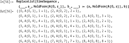
More to the point, here I do the same with the pattern that is the proxy for the buggy behavior. This shows the expressions that preceded and followed the bug.

Clearly, linearizing loses some information that was in the original output of Trace. What you lose is the information that says a certain bunch of subexpressions were triggered by some parent expression. But, the act of debugging (or indeed understanding any complex data set) is the act of suppressing extraneous information until you can identify the area where there was a problem. Then some strategically placed debug code or Print functions can often get you the rest of the way to the fix.

A very similar result to this solution can be obtained using a variation of Trace called TraceScan along with Reap-Sow. The difference is that this expression will include a bit more extraneous detail because it shows the evaluation of every symbol and constant. Here is an excerpt using Short.

   In[58]:=  Reap[TraceScan[Sow, A[2, 3]]][[2, 1]] // Short
Out[58]//Short=
             {A[2, 3], A, 2, 3, A[2 - 1, A[2, 3 - 1]], A, 2 - 1,
              Plus, 2, <<450>>, 7, 1, 8, A[0, 8], 8 + 1, Plus, 8, 1, 9}

Trace has advanced features I did not cover here. Refer to tutorial/TracingEvaluation in the Mathematica documentation for details as well as a description of the related functions TraceDialog and TracePrint.

You tried debugging using Print, but your program creates too much output too quickly and it is difficult to identify the issue. You want to have more control of the debugging process.

Mathematica has an alternative print command called PrintTemporary that inspired me to create a sort of interactive debugger. PrintTemporary works just like Print except after the evaluation is complete the output is automatically removed. Further, PrintTemporary returns a value that can be passed to the function NotebookDelete to delete the output at any time. You can get an idea of what PrintTemporary does by evaluating the following line:

In[59]:=  PrintTemporary["test"]; Pause[2]

If you could inject debug code into your ill-behaved programs that used PrintTemporary and then paused until you took some action (like pressing a button), you could effectively step though the code with the embedded prints acting like breakpoints in a real debugger. This can be done using a relatively small amount of code.

In[60]:= pmDebuggerInit[] :=
          Module[{}, $pmStep = False; $pmStop = False; CellPrint[Dynamic[Row[
               {Button["Step", $pmStep = True], Button["Stop", $pmStop = True]}]]]]
         pmWait[x__, t_] := (While[$pmStep == False && $pmStop == False,
            Pause[$TimeUnit]]; If[$pmStop, Abort[]]; NotebookDelete[t]; x)
         pmPrint[] := Module[{t}, $pmStep = False;
           t = PrintTemporary["NullSequence!!"];
           pmWait[Unevaluated[Sequence[]], t]]
         pmPrint[""] := Module[{t}, $pmStep = False;
           t = PrintTemporary["NullString!!"]; pmWait["", t]]
         pmPrint[x__] := Module[{t}, $pmStep = False;
           t = PrintTemporary[x]; pmWait[x, t]]

I explain this code further in the following "Discussion" section. For now, let’s just try it out. Here I use an instrumented version of the Ackermann function as a test example.

In[65]:=
         A[0, n_] := pmPrint[n + 1];
         A[m_, 0] := A[m - 1, 1];
         A[m_, n_] := A[m - 1, A[m, n - 1]];
         test[] := Module[{}, pmDebuggerInit[]; A[4, 1]]

Executing test[] creates the debugging controls.

The code in the solution contains two user functions, pmPrint and pmDebuggerInit. Function pmPrint has the same features as fPrint from 19.1 Printing as the First Recourse to Debugging, but it uses PrintTemporary rather than Print. Further, it calls a function pmWait, which loops and pauses until a Boolean variable becomes true. These variables are initialized in pmDebuggerInit and associated with buttons that are used to control progress of the debugging session.

Often when creating little utilities like this, it’s fun to see how far you can extend them without going too far over the top. There are a few deficiencies in the solution’s debugging techniques. First, if you insert multiple print statements, there is no way to know which one created output. Second, it would be nice if you did not always have to step one print at a time. Third, it might be nice if you can also dump the stack while the program is paused. It turns out that using a bit of cleverness can get you all this new functionality using roughly the same amount of code.

The trick here is to convert $pmStep to a counter instead of a Boolean and $pmStop to a function that can be changed by the buttons to either Abort or Print the Stack. I also introduce a new variable to collect multiple temporary print cells and move their cleanup to the button press for Step or Step 10. Finally, the pmPrint is refactored to take an optional tag to display so you can distinguish one debug output from another.

19.1 Printing as the First Recourse to Debugging, 19.3 Stack Tracing to Debug Recursive Functions, and 19.4 Taming Trace to Extract Useful Debugging Information cover some of the functions used in this recipe in more detail.

You are using various black-box numerical algorithms like FindRoot, NDSolve, NIntegrate, and the like, and you are getting puzzling results. You would like to get under the covers to gain insight into what is going on.

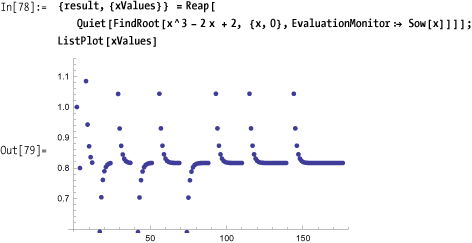
A classic problem with FindRoot (which uses Newton’s method by default) is the possibility of getting into a cycle. If you did not know about this possibility, you might be confused by the error message generated. Here I suppress the message using Quiet because I have purposefully cherry-picked a misbehaved function. FindRoot has an option EvaluationMonitor that lets you hook every call to the supplied function. Here you use Reap-Sow to capture these values for analysis. Note that you must use RuleDelayed (:>) rather than Rule (->) with EvaluationMonitor.

Sometimes a StepMonitor can also be useful for debugging. Whereas EvaluationMonitor shows each time a function is called, a StepMonitor is called only when the algorithm takes a successful step toward the solution. Stephen Wolfram explains the difference best:

In the solution example, StepMonitor is less informative than EvaluationMonitor.

One reason you might use StepMonitor during debugging is to get a sense of how much computational effort an algorithm is expending to find a solution. One measure of effort would be the average number of function calls per step. Here you can see that the effort can vary widely for different algorithms and expressions.

Evaluation and StepMonitor are also useful outside a debugging context. For example, they can be used to visualize the behavior of an algorithm for educational purposes. See the Wolfram documentation for examples.

You are a Mathematica user longing for the kinds of visual debugging environments common in mainstream programming environments like Eclipse, Visual Studio, InteliJ, DDD, and others.

Use Wolfram Workbench, a Mathematica-specific extension to the Eclipse platform. When you launch Wolfram Workbench, you must first create a project. Use menu File, New, New Project. Give the project a name. I used the name Debugging for this example. Workbench automatically creates two files named after your project. In this example, I got a Debugging.m and a Debugging.nb. The .m file is where you would enter code that you want to debug. The Debugging.nb is a normal frontend notebook file. Here you would typically set up your test calls.

Figure 19-2. Debugging.m—functions being debugged

Figure 19-3. Debugging.nb—place to exercise the functions to be debugged

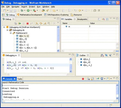
Once you have these files set up, you can place a breakpoint by double-clicking on the left margin of the line of code you want the debugger to stop. In Figure 19-4 you see a dot appear in the margin to indicate the successful placement of the breakpoint. You can place as many breakpoints as necessary.

Figure 19-4. Wolfram Workbench showing breakpoints on A[m_,0]

Now right-click on the Debugging.nb file in the Package Explorer and select Debug As... Mathematica. You will be prompted to switch to the Debug perspective, which is recommended. Figure 19-5 shows what this perspective looks like. It will also launch the frontend with Debugging.nb active. Here you can use normal Shift-Enter evaluation to execute an expression. When a breakpoint is hit, you can switch back to the Workbench to continue debugging. Here you can inspect the call stack, see the value of variables, and set further breakpoints. You can step over or into further functions using F5 (set), F6 (step over) and F7 (step return). In short, you can perform all the operations you’d expect from a modern symbolic debugger.

Figure 19-5. Wolfram Workbench in Debug perspective

Many old-time Mathematica users feel that it is sacrilegious (or perhaps just frustrating) to leave the comfortable Mathematica frontend just to debug. If you don’t have such a prejudice, your willingness will be rewarded. There is nothing like debugging within a real debugging environment! If you are a Java or C programmer who is used to such luxuries, the Eclipse-based Workbench environment is a must-have. Eclipse is an open source framework for building integrated software development environments (IDEs) that first gained popularity with Java developers. Wolfram used Eclipse to build an alternative development environment for Mathematica as an alternative to the traditional frontend. However, you don’t need to abandon the traditional Mathematica interface to use Workbench to debug. In this section, I refer to Eclipse when speaking about generic features that are true about all Eclipse IDEs and Workbench when speaking about features of Workbench in particular.

If you have never used more traditional languages, such as Java, C, C++ and C#, then you are likely to find working in Workbench somewhat foreign. To avoid being frustrated, you should keep a few ideas in mind. First, because Workbench is built on top of Eclipse and Eclipse was built outside of Wolfram, you should not expect Workbench to have the same look and feel as the traditional frontend. You should approach it as you would approach any new piece of software—with an open mind and no preconceptions. For example, you should not expect to debug code that is written using all the fancy mathematical typesetting features available in a notebook. If you developed code solely using the .nb format, you should save your code as a .m, which is a pure text format. This is not to say you can’t launch notebooks from Eclipse (the solution shows this is possible) but rather you should make all code that you wish to debug available in text format.

Another important concept of Eclipse is that it wants to manage all the source code under a project. Projects in Eclipse typically correspond to directories under a specific root directory you choose when Eclipse is installed. It is possible to specify other directories outside this hierarchy, but you will not automatically pick up files that happen to be in an existing location. You can use File, Import for that purpose.

In addition to source code-level breakpoints, Workbench supports message breakpoints that break when a function emits any error message and symbol breakpoints that provide a convenient way to place a breakpoint on an overloaded function name. For example, a symbol breakpoint can be used to put a break on all three variants of the Ackermann function A. The three types of breakpoints are accessible from the Breakpoints tab shown in Figure 19-6. The message break is set using , and is used for symbol breakpoints. There are also buttons for clearing selected breakpoints, , or all breakpoints, , and you can uncheck a breakpoint in the list to temporarily disable it.

Figure 19-6. Breakpoints tab has toolbar buttons for setting various types of breakpoints

If you are new to Eclipse, you should definitely check out the series of screencasts on Wolfram Workbench at http://bit.ly/2srUoi .

You want to write unit tests to help uncover bugs in a library of functions. Perhaps you are familiar with the unit-testing frameworks that exist in other languages, and you would like the equivalent for Mathematica.

Wolfram Workbench is nicely integrated with MUnit, a unit-testing framework for Mathematica. You create a unit test in a special file with extension .mt. The easiest way to create such a file is to right-click on your project and select New, Mathematica Test File (you should make sure you are in Mathematica Development Perspective, or you will have to navigate into the Other submenu to get to this feature).

The most convenient way to create your first test case is to type Test and then hit Ctrl-Space to trigger code assist, which automatically creates the test boilerplate.

(*Mathematica test file for Ackermann*)
Test[
    A[0,0]

    ,
    1

    ,
    TestID->"Test2-20090508-O1L1K5"
]

Test[
    A[1,0]

    ,
    2

    ,
    TestID->"Test2-20090508-N4W7U7"

]

Test[
    A[0,1]

    ,
    2

    ,
    TestID->"Test2-20090508-F5F9A7"

]

(*This test will fail!*)
Test[
    A[1,2]

    ,
    3

    ,
    TestID->"Test2-20090508-L7N0S2"
]

You can execute your unit tests at any time by saving the test file, right-clicking on it in the package explorer, and selecting Run As, Mathematica Test. This will generate a Test Report, as shown in Figure 19-7. The report shows which tests passed and which failed. Unique TestIDs are essential to this function, and Workbench has a feature that will help fix and duplicate IDs. Simply right-click on the file, select the Source menu, and then select Fix Test IDs.

Figure 19-7. Test report generated after running the tests defined in the solution

Functions like Ackermann that return scalar values are easy to inspect in the failed tests section to investigate the difference between the expected and actual output. In Figure 19-7, you can see that the expected output is 6, but the actual output is 4. In this case, it is the test function that is wrong, because the correct output is 4. The more typical circumstance is that the function is wrong, but in either case you can quickly see that something is awry. With more complex outputs, it can be difficult to find the difference. A useful feature of Workbench is Failure Compare. Simply right-click on the failure test ID and select Failure Compare. This will open a dialog with a side-by-side tree view of the expected and actual expression (see Figure 19-8). You can expand the tree to inspect the branches that indicate differences (the X).

Figure 19-8. Use the test failure comparator to drill down into test results to detect problems

See the Wolfram Workbench unit-testing screencast at http://bit.ly/dOJBL for a step-by-step overview of unit testing.

Although the MUnit Test function is easy to use, it is not the most appropriate function for certain types of testing. For example, you may want to define your test in terms of pattern matching.

MUnit provides other test functions, including TestMatch, TestFree, TestStringMatch, and TestStringFree. TestMatch uses MatchQ to compare actual and expected results, and TestFree uses FreeQ. Likewise, TestStringMatch uses StringMatchQ, and TestStringFree uses StringFreeQ.

TestMatch[
    {1,2,3,4,5}
    ,
    {Integer}
    ,
    TestID->"TestOther-20090509-L8U9H1"
]

TestFree[
    {10,12,1/2,2/3,3/4,4/5,5/6}
    ,
    {__Complex}
    ,
    TestID->"TestOther-20090509-L8U9H2"
]

TestStringMatch[
    "Hello"
    ,
    "H" ~~ __ ~~ "o"
    ,
    TestID->"TestOther-20090509-L8U9H3"
]

TestStringFree[
    "Hello"

    ,
    "x"
    ,
    TestID->"TestOther-20090509-L8U9H4"
]

You can create even more flexible tests by using the EquivalenceFunction option of Test to specify an alternative definition of success. The following test succeeds if the actual value is greater than 0.

Test[Cos[1]^2 + Sin[1]^2 - Sqrt[1 - Exp[-10]],
  0,
  EquivalenceFunction -> Greater,
  TestID -> "ID17"]

This option comes in handy when you are creating tests where exact equality is not useful. For example, you might want to use Round or Chop before comparing.

Test[
InverseFourier[Fourier[{2, 1, 1, 0, 0, 0}]],
  {2, 1, 1, 0, 0, 0},
  EquivalenceFunction -> (Chop[#1] == Chop[#2] &),
  TestID -> "ID42"
  ]

Of course, you can just as readily write the test with Chop applied to the actual computation, but I feel that EquivalenceFunction better documents the test designer’s intention. Another example is when you are only worried about equality up to a specified tolerance.

Test[
(12/7) (2 Sqrt[2] - 1),
  Pi,
  EquivalenceFunction -> Abs[#1-#2] < 0.01,
  TestID -> "ID66"

You have a complex test suite with many tests. The tests may naturally group into sections. Further, you want the ability to turn on and off test sections as well as state dependencies between sections, possibly to account for side effects. For example, you want to say, "only continue with this section if tests succeed, because further tests rely on results computed by earlier tests."

There are a few advanced MUnit features that are useful for organizing tests and managing test dependencies. You can organize tests into sections using BeginTestSection[name,switch] and EndTestSection[].

(*Switches to activate and deactivate sections*)
Sect1Active = True;
Sect2Active = True;

(*Section 1*)
BeginTestSection["sect1", Sect1Active]

(*All tests in this section depend on first test success.*)
TestFree[str=OpenRead["SomeTestFile.txt"], $Failed,
EquivalenceFunction ->UnsameQ,
TestID-> "TestAdvanced-20090509-060603", TestFailureAction -> "SkipSection"]

Test[Read[str, Number], 5, TestID -> "IDS1_1"]

Test[Read[str, Word], "cars", TestID -> "IDS1_2"]

EndTestSection[]

(*Section 2*)
BeginTestSection["sect2", Sect2Active]
Test[2 + 2, 4, TestID -> "IDS2_1"]
EndTestSection[]

If it does not make sense to continue tests after a failure, you can also specify TestFailureAction "Abort". This feature is available even if you do not use sections.

If you have a complex Mathematica library, you will want to organize it into separate test files. However, running each test separately would be tedious, so MUnit provides a TestSuite construct. First, you should place all your test files (.mt files) into a folder under the main project folder. Then create a test file that ties all the tests together into a suite, as shown in Figure 19-9.

Figure 19-9. TestSuite is a test file that allows you to run other test files all at once

You would like to create unit tests but you prefer to work in the traditional frontend rather than Workbench.

You need a test driver to run the tests. This mimics the basic functionality of Workbench.

In[88]:= Needs["MUnit`"];
         TestDriver[tests__] :=
          Module[{testList = {tests}, numTests, failedTests},
           numTests = Length[testList];
           failedTests = Select[{tests}, (FailureMode[#] =!= "Success") &];
           Print["Passed Tests: ", numTests - Length[failedTests]];
           Print["Failed Tests: ", Length[failedTests]];
           Print["Failed Test Id: ", TestID[#], "
Expected: ",
              ExpectedOutput[#], " Actual: ", ActualOutput[#]] & /@ failedTests;
          ]

Note

The MUnit package is not part of Mathematica 7, but you can still use it if you have installed Wolfram Workbench 1.1 or higher. You need to tell the kernel where to find the package. This will vary from system to system, but generally it will be under the Wolfram Research directory where Mathematica is installed. You want to find a directory called MUnit and add the path to that directory to $Path. On my Windows XP installation, I added the location to $Path by executing:

In[90]:= AppendTo[$Path, FileNameJoin[{"C:", "Program Files",
            "Wolfram Research", "WolframWorkbench", "1.1", "plug-ins",
            "com.wolfram.eclipse.testing_1.1.0", "MathematicaSource"}]]

Out[90]= {C:Program FilesWolfram
            ResearchMathematica7.0SystemFilesLinks,
          C:UsersSal ManganoAppDataRoamingMathematicaKernel,
          C:UsersSal ManganoAppDataRoamingMathematicaAutoload,
          C:UsersSal ManganoAppDataRoamingMathematicaApplications,
          C:ProgramDataMathematicaKernel,
          C:ProgramDataMathematicaAutoload,
          C:ProgramDataMathematicaApplications, .,
          C:UsersSal Mangano, C:Program FilesWolfram
            ResearchMathematica7.0AddOnsPackages,
          C:Program FilesWolfram
            ResearchMathematica7.0AddOnsLegacyPackages,
          C:Program FilesWolfram
            ResearchMathematica7.0SystemFilesAutoload, C:Program
            FilesWolfram ResearchMathematica7.0AddOnsAutoload,
          C:Program FilesWolfram
            ResearchMathematica7.0AddOnsApplications, C:Program
            FilesWolfram ResearchMathematica7.0AddOnsExtraPackages,
          C:Program FilesWolfram
            ResearchMathematica7.0SystemFilesKernelPackages,
          C:Program FilesWolfram
            ResearchMathematica7.0DocumentationEnglishSystem,
          C:Program FilesWolfram
            ResearchWolframWorkbench1.1plug-inscom.wolfram.eclipse.
            testing_1.1.0MathematicaSource}

You can add this to init.m if you intend to use MUnit frequently. Alternatively, you can also copy the MUnit package into one of the locations in $Path.

Here is a simple example of using the driver. I purposefully made tests with ID2 and ID4 fail.

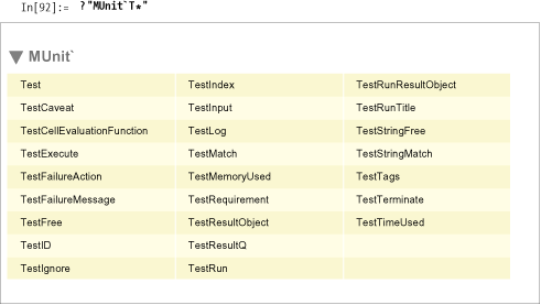
The test driver used in the preceding "Solution" section is very basic and does not support all the features available when you build unit tests in Workbench. If you are ambitious, you can build a more sophisticated driver—even one that has more features than Workbench. It really depends on your needs. The main requirement is to become familiar with the MUnit API. Although documentation on MUnit is sparse at the time I am writing this, well-written Mathematica packages are self-describing. For example, you can find all the public functions in the package by using ?"MUnit`*". For the sake of space, I’ll only list the functions that begin with the letter T. By clicking on the output, you can see what the function or option does. The most important functions are selectors, like TestID, because these allow you to extract information from a TestResultObject, which is the output produced by functions like Test, TestMatch, and so on.

By inspecting MUnit's functions, I was inspired to create a test driver that supports the idea of test sections (see 19.10 Organizing and Controlling MUnit Tests and Test Suites). However, instead of a BeginTestSectionEndTestSection pair, I use a single TestSection function. The TestDriver will work with multiple TestSections or multiple Tests but not mixtures of both. For this driver to handle skipping and aborting, it must be careful to evaluate a test lazily, hence, it uses Hold and the HoldAll attribute judiciously. It also uses Catch and Throw combinations. This is a feature of Mathematica I have largely avoided in the book, but it sometimes comes in handy as a way to terminate an iteration without cumbersome conditional logic. In this case, the function RunTest causes a test to evaluate and tests for failure. If the test does not succeed, it defers further decisions to OnFailedTest based on the test’s FailureMode. OnFailedTest will either Throw or return, depending on the mode. Further, it uses the mode as a tag in the Throw, so the appropriate Catch handler can intercept the failure.

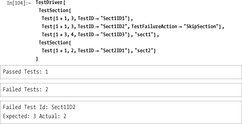
In[93]:= ClearAll[TestDriver, TestSection, RunTest, OnFailedTest];
         SetAttributes[{TestDriver, TestDriver2, TestSection, RunTest}, HoldAll];

         (*OnFailedTest simply returns the test if mode is Continue,
         otherwise it throws using mode as a tag.*)
         OnFailedTest[test_, "Continue"] := test
         OnFailedTest[test_, mode_] := Throw[test, mode]

         (*RunTest tests the failure mode and updates
          counters. It defers failure action to OnFailedTest.*)
         RunTest[testTestResultObject] :=
          If[FailureMode[test] =!= "Success", failedTests++;
           OnFailedTest[test, TestFailureAction[test]], passedTests++; test]

         (*A TestSection has one or more tests, a name,
         and Boolean for enabling or disabling the section.*)
         TestSection[tests__, section_String, False] := {}
         TestSection[tests__, section_String, _ : True] :=
          Module[{},
           Catch[ReleaseHold[RunTest[#] & /@ Hold[tests]], "SkipSection"]]

         (*TestDriver2 valuates the results of tests.*)
         TestDriver2 [tests__] := Module [{testList = {tests}, numTests, failed},
           failed =Select[{tests}, (FailureMode [#] =!= "Success") &];
           Print["Passed Tests: ", passedTests];
           Print["Failed Tests: ", failedTests];
           Print["Failed Test Id: ", TestID[#], "
Expected: ",
              ExpectedOutput[#], " Actual: ", ActualOutput [#]]& /@ failed;
         ]

        (*This instance of TestDriver executes sections.*)
        TestDriver[secs__TestSection] :=
         Block[{ passedTests = 0, failedTests = 0},
          TestDriver2 @@ Flatten[{Catch[ {secs}, "Abort"]}]]

        (*This instance of TestDriver executes tests.*)
        TestDriver[tests__] := Block[{passedTests = 0, failedTests = 0},
          TestDriver2 @@ Flatten[{Catch[RunTest /@ {tests}, "Abort"]}]]

Here I put the driver through its paces demonstrating different failure scenarios.

In this scenario, the second test in sectl fails with an Abort; hence, tests with test IDs "Sect1ID3" and "Sect2ID1" are not run.

In this scenario, the second test in sectl fails with a "SkipSection"; hence, the test with test ID "Sect1ID3" is skipped, but a "Sect2ID1" runs.

Here sections are not used, but a TestFailureAction of "Abort" is still handled appropriately.

The concept of test sections is native to MUnit when used with Workbench, but has a different syntax. This is covered in 19.10 Organizing and Controlling MUnit Tests and Test Suites.