You want to perform common statistical analysis of data sets. These metrics represent the entry-level statistical functions that all users of Mathematica should have under their belts.

It should come as little surprise that Mathematica is equipped with the standard statistical functions. Here I use the byte count of Mathematica files on my folder as a source of data.

In[1]:=  data = N[ FileByteCount /@
             FileNames[FileNameJoin[{NotebookDirectory[],"*.nb"}]]];
         (*Compute the mean.*)
         Mean[data]
Out[2]=  2.45023 × 106

The statistical functions you will use most in Mathematica (Mean, Median, Max, Min, Variance, and StandardDeviation) have obvious names and obvious uses. Here I get a bit fancy by computing a table in one step by using Through with the list of functions.

Not quite as pedestrian, quantiles are a common concept in statistics that generalizes the concept of median to other subdivisions.

In[4]:=  (*Find the lower quantile.*)
         Quantile[data, 1/4]
Out[4]=  14412.

In[5]:=  (*Find the 1/2, 1/3, 1/4, ... 1/10.*)
         Quantile[data, #] & /@ Table[1/n, {n, 2, 10}]
Out[5]=  {114698., 26623., 14412., 7712., 6102., 5456., 4775., 3865., 3514.}

In[6]:=  Quantile[data, 1/2]
Out[6]=  114698.

When used with default parameters Quantile always returns some element in the actual list. Thus, Quantile[data, 1/2] may not be the same as Median.

In[7]:=  Quantile[data, 1/2] == Median[data]
Out[7]=  True

With the following parameters, Quantile and Median are identical. See Quantile documentation for the meaning of these parameters.

In[8]:=  Quantile[data, 1/2, {{1/2,0}, {0,1}}] == Median[data]
Out[8]=  True

The basic functions covered in the solution are no doubt familiar and hardly warrant further elaboration except to note their generality.

All of the statistics functions in Mathematica work with SparseArray, which is very convenient when you have a very large but sparse data set.

Further, given Mathematica’s symbolic nature, you should not be too surprised that it can do more than other common data analysis applications, such as MS Excel.

What does this result mean? It is the formula for computing the variance of a set of data with 3 a’s, 1 b, 2 c’s and 2 d’s. You can use this formula using ReplaceAll.

This is exactly the result you would get if you took the direct route.

This may seem completely academic; for many of you, it will be so. Yet consider that symbolic form allows you to perform further symbolic manipulations that account for properties you may know about the symbolic data. For example, imagine the items were all angles in radians in a given relationship and you wanted to know the formula for the variance of their sine. Such examples are contrived only until you need to do a similar transformation.

These symbolic capabilities also imply you can use these functions with common distributions rather than on individual values.

Another common statistical metric is the mode. This function is called Commonest in Mathematica and can be used to find the commonest or the n commonest. Related to this is a new function in version 7, Tally, that gives the individual counts.

In[16]:=  list = First[ RealDigits[Pi, 10, 50]];

In[17]:=  {Commonest[list], Commonest[list, 3]}
Out[17]=  {{3}, {3, 1, 9}}

In[18]:=  Tally[list]
Out[18]=  {{3, 9}, {1, 5}, {4, 4}, {5, 5}, {9, 8}, {2, 5}, {6, 4}, {8, 5}, {7, 4}, {0, 1}}

There is a multivariate statistics package (see MultivariateStatistics/guide/Multivariate StatisticsPackage) that generalizes notions of mean, median, and so on, to multiple dimensions. Here you will find functions such as SpatialMedian, SimplexMedian, and PolytopeQuantile, which clearly are targeted at specialists.

You want to generate random numbers that have nonuniform distributions. Many recipes in this book use RandomReal and RandomInteger, but these functions give uniform distributions unless you specify otherwise.

Both RandomReal and RandomInteger can take a distribution as their first argument. RandomReal uses continuous distributions, including NormalDistribution, HalfNormalDistribution, LogNormalDistribution, InverseGaussianDistribution, GammaDistribution, ChiSquareDistribution, and others. RandomInteger uses discrete distributions, such as BernoulliDistribution, GeometricDistribution, HypergeometricDistribution, PoissonDistribution, and others.

In[19]:=  RandomReal[NormalDistribution[], 10]
Out[19]=  {-0.96524, 1.19926, 0.989088, 0.156427, -0.336326,
           -1.66671, 0.149802, -0.464219, -0.998164, 0.948215}

In[20]:=  RandomInteger[PoissonDistribution[5], 10]
Out[20]=  {5, 2, 6, 5, 6, 4, 3, 4, 4, 5}

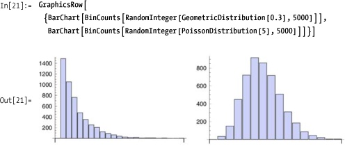
You can visualize distributions using BinCounts and BarChart.

Another way to visualize the various continuous distributions is to generate a random raster using each distribution. How would you rewrite this to remove the redundancy? (Hint: functional programming!)

Other useful functions to explore in the Mathematica documentation are SeedRandom, BlockRandom, and RandomComplex.

See 12.12 Hypothesis Testing with Categorical Data for a common method for testing random generators based on the chi-square distribution.

You want to compute the probability density function (PDF) and cumulative density function (CDF) of various distributions. You may also want to determine the characteristic function of the associated distribution.

Use PDF to compute the probability density function and CDF to compute the cumulative density function. I illustrate the use of these functions using the standardized normal distribution (mean 0 and variance 1).

The CDF is obtained from the PDF by integrating the PDF from –∞ to x, which you can illustrate in Mathematica very easily. The implementation given here is designed to execute the integration only once and then store it as a new function for subsequent evaluation, so it is almost as fast as the built-in CDF. There is no compelling reason to use this over the built-in CDF implementation. It is here strictly as an illustration of the relationship. If you use Mathematica to teach statistics, it is a good idea to peek under the covers of black box functions like CDF whenever possible.

Clearly, you can also obtain the closed-form formula for the CDF of any particular distribution.

Find the value at –∞.

So the closed-form value for the CDF of the normal distribution is

In[29]:=  cumNormDist[x_] := Erf[x/Sqrt[2]]/2 + 0.5

The classic application of a PDF is in computing the probability that a particular value falls within some range. For example, consider the probability of a value falling between 0 and 0.25 for various distributions.

In[30]:=  Integrate[PDF[#, x], {x, 0, 0.25}] & /@
           {UniformDistribution[{0, 1}], NormalDistribution[0, 1],
            HalfNormalDistribution[1], ChiSquareDistribution[2]}
Out[30]=  {0.25, 0.0987063, 0.158106, 0.117503}

Based on the definition of the CDF, it is easy to see that it computes the probability that a value will be less than or equal to a specific value. Subtracting the CDF from 1 will give the probability of a value being greater than a specified limit.

In[31]:=  (*Probability that a normally distributed random variable will
           be less than or equal to 0.5*)CDF[NormalDistribution[0, 1], 0.5]
Out[31]=  0.691462

In[32]:=  (*Probability that a normally distributed random variable will
           be greater than 0.8*)1 - CDF[NormalDistribution[0,1], 0.8]
Out[32]=  0.211855

In[33]:=  (*Probability that a normally distributed random
            variable will be less than -1 or greater than 1*)
          CDF[NormalDistribution[0,1], -1.] +
           (1 - CDF[NormalDistribution[0,1], 1.])
Out[33]=  0.317311

When you plot a PDF, you can use ColorFunction to highlight regions of interest, but make sure you also set Filling Axis and ColorFunctionScaling False. Here I plot the regions of interest whose total area (and hence probability) is approximately 0.317311.

Use CharacteristicFunction[dist,var] to extract the characteristic function of a distribution in terms of a variable var. Here are the functions for five common distributions.

12.12 Hypothesis Testing with Categorical Data demonstrates an application of the chi-square distribution.

12.6 Measuring the Shape of Data demonstrates metrics for capturing the shapes of various distributions.

You want to illustrate the central limit theorem (CLT) to yourself or your students.

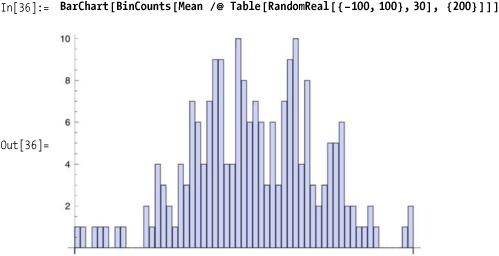
The CLT states that the mean of sufficiently large samples from any distribution will approximate a normal distribution. You can illustrate this by averaging suitably large random samples from a nonnormal distribution, such as the uniform distribution.

The CLT is often stated in a very technical way. In Statistics in a Nutshell, Boslaugh and Watters explain that the CLT "states that the sampling distribution of the sample mean approximates the normal distribution, regardless of the distribution of the population from which samples are drawn, if the sample size is sufficiently large" (137). Other references define it in an equally technical way. The solution shows that the concept is not difficult, although the result is certainly not obvious. The solution demonstrates 200 samples of uniformly generated lists of random numbers, each of length 30, being averaged and then the counts of each integer-valued range being organized into bins and plotted. The shape looks roughly normal, which is the prediction of the CLT. BinCounts, Mean, and RandomReal are relatively easy to understand (see prior recipes), so this makes the idea behind the CLT rather concrete.

To further emphasize that this is not a property of the uniform distribution, you can substitute other distributions. These use finer grained bins due to the tighter range of numbers generated, but the result is similar. As an exercise, wrap a Manipulate around the code in the "Solution" section above and adjust both the sample size and the number of samples. This will illustrate that the validity of the CLT is predicated on a sufficiently large number of samples of sufficiently large size.

A proof of the CLT can be found at Wolfram MathWorld: http://bit.ly/S00Y1 .

You want to measure the relationship between data sets to see if they vary about the mean in a similar way (covariance) or if there is a linear relationship (correlation).

Covariance and Correlation both operate on matrices. If you pass a single matrix, it will return a covariance (or correlation) matrix resulting from computing the covariance between each column. To demonstrate this clearly, I’ll engineer a matrix with an obvious relationship between the first and second column and a weak correlation of these in a third column. The output matrix will always be symmetrical. The correlation matrix will always have ones on the diagonal, since these entries represent correlations of columns with themselves. You can also pass two matrices, in which case you get the covariance (or correlation) with respective columns.

   In[40]:=  SeedRandom[2];
             (data = Transpose[{{0, 1, 2, 3, 4, 5, 6, 7, 8, 9},
                   {0, 10, 20, 30, 40, 50, 60, 70, 80, 90},
                   RandomReal[{-1, 1}, 10]}]) // TableForm
Out[41]//TableForm=
             0 0  0.44448
             1 10 -0.781103
             2 20 -0.0585946
             3 30 0.0711637
             4 40 0.166355
             5 50 -0.412115
             6 60 -0.669691
             7 70 0.202516
             8 80 0.508435
             9 90 0.542246

   In[42]:=  Covariance[data] // TableForm
Out[42]//TableForm=
             9.16667  91.6667 0.467288
             91.6667  916.667 4.67288
             0.467288 4.67288 0.228412

   In[43]:=  Correlation[data] // TableForm
Out[43]//TableForm=
             1.       1.       0.322938
             1.       1.       0.322938
             0.322938 0.322938 1.

   In[44]:=  Correlation[data, data^2] // TableForm
Out[44]//TableForm=
             0.962691 0.962691 0.00604923
             0.962691 0.962691 0.00604923
             0.442467 0.442467 -0.522003

You want to summarize the shape of your data using some common statistical measures.

Use Skewness to measure the asymmetry of a distribution. A symmetrical distribution like the NormalDistribution will have skewness of zero. A positive skewness indicates the right tail is longer, while a negative skewness indicates the left tail is longer.

Use QuartileSkewness to measure if the median is closer to the upper or lower quartile. QuartileSkewness is a more robust measure of skewness in the presence of extreme values.

In[47]:=  data = {0.1, 0.3, 0.7, 1, 0.6, 99, 0.8, 2, 2.1, 0.95, 1.7, 0.69};
          {QuartileSkewness[data], Skewness[data]}
Out[48]=  {0.618257, 3.01242}

Use Kurtosis to measure the sharpness of the peak of a distribution. A high kurtosis distribution has a sharper peak and longer, fatter tails, whereas a low kurtosis distribution has a more rounded peak and shorter, thinner tails.

CentralMoment is a fundamental measure that underlies statistical measures of shape. It is computed as

The second central moment of a data set is called the population variance (which is not as commonly used as sample variance as computed by the Variance function).

In[50]:=  data = {0.1, 0.3, 0.7, 1, 0.6, 99, 0.8, 2, 2.1, 0.95, 1.7, 0.69};

In[51]:=  Table[CentralMoment[data, i], {i, 1, 3}]
Out[51]=  {1.77636 × 10–15, 734.086, 59915.}

Skewness is equivalent to CentralMoment[list,3]/CentralMoment[list,2]^(3/2); Kurtosis is CentralMoment[list,4]/CentralMoment[list,2]^2.

You have a large data set and you want to identify outliers and possibly adjust the statistics to compensate.

A simple way to identify outliers is to use Sort and inspect the beginning and end of the list. You can also look at a certain number of elements near the minimum and maximum using Nearest.

In[52]:=  data = Join[{0.0001, 0.0005}, RandomReal[{10, 30}, 500], {1000, 1007}];
           {min, max} = {Min[data], Max[data]};
          {Nearest[data, min, 5], Nearest[data, max, 5]}
Out[54]=  {{0.0001, 0.0005, 10.0021, 10.1101, 10.1403},
           {1007, 1000, 29.9915, 29.9773, 29.975}}

You can also compute the trimmed mean, which is the mean after dropping a fraction of the smallest and largest elements.

In[55]:=  {Mean[data], TrimmedMean[data, 0.2]}
Out[55]=  {24.0623, 20.173}

Here I take advantage of a feature of Tally that allows you to provide custom equivalence function. The idea here is to treat values within a specified distance of each other as equal. In this case, I use distance 5. This shows that there are 3 clusters of values in the data and some outliers with low frequency of occurrence.

   In[56]:=  Tally[data, (Abs[#1 - #2] < 5) &] //TableForm
Out[56]//TableForm=
             0.0001  2
             25.5715 235
             10.4722 135
             17.0082 130
             1000    1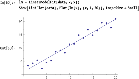
             1007    1

You have a data set and would like to find a linear model of the data. A linear model is commonly called a "linear regression." A linear model has various statistics that define its accuracy, and you typically want to obtain these as well.

In[57]:= data = Table[{x, x + RandomReal[{-2, 3}]}, {x, 1, 20}];

Use Fit in versions prior to Mathematica 7.

Use LinearModelFit in version 7 and above to build a linear model that you can then use to plot or extract statistics.

LinearModelFit is a vast improvement over Fit since it is not just a way to synthesize a function. Once you have constructed a linear model, you can query its various properties, of which there are quite a few. To find out what is available, simply ask the model. Ask for a specific property by name.

In[62]:=  lm["Properties"]
Out[62]=  {AdjustedRSquared, AIC, ANOVATable, ANOVATableDegreesOfFreedom,
           ANOVATableEntries, ANOVATableFStatistics, ANOVATableMeanSquares,
           ANOVATablePValues, ANOVATableSumsOfSquares, BetaDifferences, BestFit,
           BestFitParameters, BIC, CatcherMatrix, CoefficientOfVariation,
           CookDistances, CorrelationMatrix, CovarianceMatrix, CovarianceRatios,
           Data, DesignMatrix, DurbinWatsonD, EigenstructureTable,
           EigenstructureTableEigenvalues, EigenstructureTableEntries,
           EigenstructureTableIndexes, EigenstructureTablePartitions,
           EstimatedVariance, FitDifferences, FitResiduals, Function,
           FVarianceRatios, HatDiagonal, MeanPredictionBands,
           MeanPredictionConfidenceIntervals, MeanPredictionConfidenceIntervalTable,
           MeanPredictionConfidenceIntervalTableEntries, MeanPredictionErrors,
           ParameterConfidenceIntervals, ParameterConfidenceIntervalTable,
           ParameterConfidenceIntervalTableEntries, ParameterConfidenceRegion,
           ParameterErrors, ParameterPValues, ParameterTable, ParameterTableEntries,
           ParameterTStatistics, PartialSumOfSquares, PredictedResponse, Properties,
           Response, RSquared, SequentialSumOfSquares, SingleDeletionVariances,
           SinglePredictionBands, SinglePredictionConfidenceIntervals,
           SinglePredictionConfidenceIntervalTable,
           SinglePredictionConfidenceIntervalTableEntries, SinglePredictionErrors,
           StandardizedResiduals, StudentizedResiduals, VarianceInflationFactors}

In[63]:=  lm["RSquared"]
Out[63]=  0.944788

In[64]:=  lm["MeanPredictionErrors"]
Out[64]=  {0.627101, 0.579603, 0.533846, 0.490318, 0.449667, 0.412744,
           0.380636, 0.354652, 0.336216, 0.326608, 0.326608, 0.336216, 0.354652,
           0.380636, 0.412744, 0.449667, 0.490318, 0.533846, 0.579603, 0.627101}

In[65]:=  lm["BestFit"]
Out[65]=  0.981879 + 0.990357 ×

You can also get the best Fit function by using Normal.

In[66]:=  Normal[lm]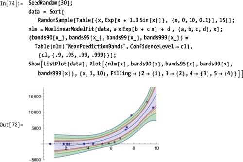
Out[66]=  0.981879 + 0.990357 ×

FindFit and LeastSquares are other related functions you can explore in the Mathematica documentation.

GeneralizedLinearModelFit and DesignMatrix are Mathematica 7 functions that are also worth exploring in the documentation and tutorials.

You want to fit data to a function for which you have knowledge of the mathematical model. Specifically, you know the model is nonlinear and, hence, neither Fit nor LinearModelFit is appropriate.

Use FindFit in versions prior to Mathematica 7.

Use NonLinearModel fit in Mathematica 7 as a more complete solution.

As with LinearModelFit, NonlinearModelFit encapsulates a wealth of information.

In[73]:=  nlm["Properties"]
Out[73]=  {AdjustedRSquared, AIC, ANOVATable, ANOVATableDegreesOfFreedom,
           ANOVATableEntries, ANOVATableMeanSquares, ANOVATableSumsOfSquares,
           BestFit, BestFitParameters, BIC, CorrelationMatrix, CovarianceMatrix,
           CurvatureConfidenceRegion, Data, EstimatedVariance, FitCurvatureTable,
           FitCurvatureTableEntries, FitResiduals, Function, HatDiagonal,
           MaxIntrinsicCurvature, MaxParameterEffectsCurvature, MeanPredictionBands,
           MeanPredictionConfidenceIntervals, MeanPredictionConfidenceIntervalTable,
           MeanPredictionConfidenceIntervalTableEntries,
           MeanPredictionErrors, ParameterBias, ParameterConfidenceIntervals,
           ParameterConfidenceIntervalTable, ParameterConfidenceIntervalTableEntries,
           ParameterConfidenceRegion, ParameterErrors, ParameterPValues,
           ParameterTable, ParameterTableEntries, ParameterTStatistics,
           PredictedResponse, Properties, Response, RSquared, SingleDeletionVariances,
           SinglePredictionBands, SinglePredictionConfidenceIntervals,
           SinglePredictionConfidenceIntervalTable,
           SinglePredictionConfidenceIntervalTableEntries,
           SinglePredictionErrors, StandardizedResiduals, StudentizedResiduals}

For example, you can extract and plot confidence bands for various confidence levels.

Or you can extract a variety of statistics.

The statistical model analysis guide (guide/StatisticalModelAnalysis) is a good starting point for exploring all the new modeling capabilities in Mathematica 7.

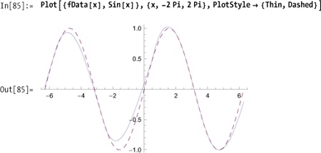
You have a set of data points and want to construct a function you can use to predict values at other points.

Normally, you would interpolate data that was obtained in the wild without any a priori notion of the underlying function. However, as a simple illustration, I’ll sample data from a known function.

In[82]:=  xvalues = Sort[RandomReal[{-4 Pi, 4 Pi}, 18]];
          data = Table[{x, Sin[x]}, {x, xvalues}];
          fData = Interpolation[data]
Out[84]=  InterpolatingFunction[{{-11.3374, 12.5436}}, <>]

Interpolation returns an InterpolationFunctionObject, which can be used just like a normal function. The default order for Interpolation is 3 but this can be varied using the option InterpolationOrder.

You have experimental data suggesting a linear relationship between an independent and dependent variables; however, you are unsure if the relationship is causal. You run an experiment using an experimental group and a control group. You want to know if the results of the experiment are statistically significant.

Analysis of variance (ANOVA) is a popular statistical technique that is very important in the analysis of experimental results. Mathematica provides this functionality in a package aptly named ANOVA`. To illustrate the use of this package, I borrow a toy example from Boslaugh and Watters’ Statistics in a Nutshell. Imagine you collected the data in table coffeeIQ suggesting a relationship between coffee consumption in cups and IQ as measured by some standardized IQ test.

The question that remains is whether there is a causal relationship between caffeine and IQ, since one could equally suppose smart people just like to drink coffee. To investigate further, you design an experiment with two randomly selected groups: everyone in the first group receives a caffeine pill, and those in the second group receive a placebo. The pills are administered in a double-blind method, at the same time, under the exact same conditions, and each group is administered an IQ test at a specific time after the pills were taken. From these experiments you obtain the following data, where the first entry is 1 for those who received the caffeine and 0 for those who received the placebo. The second entry is the measured IQ.

In[94]:=  experiments = {{1, 110}, {1, 100}, {1, 120}, {1, 125}, {1, 120}, {1, 120},
             {1, 115}, {1, 98}, {1, 95}, {1, 91}, {0, 100}, {0, 95}, {0, 100},
             {0, 122}, {0, 115}, {0, 88}, {0, 97}, {0, 87}, {0, 92}, {0, 76}};

Using ANOVA you see

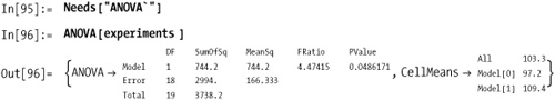
Here the important results are the FRatio (higher is better) and PValue (smaller is better). The PValue is the probability of obtaining the result at least as extreme as the one that was actually observed, given that the null hypothesis is true. Typically one will reject the null hypothesis when the PValue is less than 0.05.

You may wonder why the output of ANOVA is formatted as it is. Here Mathematica is emulating a popular statistics package called Minitab. You can drill down to the raw values easily enough.

In[97]:=  (ANOVA /. ANOVA[experiments ])[[1]]
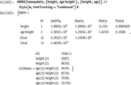
Out[97]=  {{1, 744.2, 744.2, 4.47415, 0.0486171}, {18, 2994., 166.333}, {19, 3738.2}}

The solution shows a one-way ANOVA. It is frequently the case that there are multiple independent variables. In this case, you must describe the model and variables more precisely. For example, suppose you were measuring height and age of men as a predictor of income. For the purpose of this experiment, we will designate men under 5’10" as "short," assigning them height classification 1 and "tall" men classification 2. Similarly, we will define "young" men as under 40 with age classification 1 and "mature" men with age classification 2.

Here I use All in the model input to indicate I want to analyze all products of the main effects. You can also specify the products individually. For example, if you want to analyze the significance of height and height and age together, you can specify the model parameter as {height, age height}.

There are a few standard post hoc tests you can run to determine which group’s means were significantly different given SignificanceLevel (default is 0.05). I will not delve into the statistics behind these tests. You should refer to one of the resources in the See Also section. The output is fairly self-explanatory. Here we see that using the Bonferroni and Tukey tests, variation in income due to height was statistically significant between groups 1 and 2, but age did not show up as significant for either test.

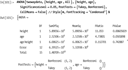
Returning to the data from the Solution section, we can see how the tests can pass at one significance level but fail at a tighter tolerance. Note also how I use the output as a replacement rule to extract only the test results.

In the examples given here, I have also used the option CellMeans False, which suppresses the display of the means.

Basic information on ANOVA can be found on Wikipedia at http:/bit.ly/bf8PrO, and in Boslaugh and Watters, Statistics in a Nutshell.

You want to determine if there are statistically significant relationships within categorical data.

The chi-square test is a standard computation on categorical data. Categorical data is that for which the response is a choice among a set of discrete categories rather than a measurement on a continuous scale. Common examples are sex {male, female}, party {Democrat, Republican}, or sometimes data that could be placed on a scale but for simplicity is lumped into discrete groups, for example, blood pressure {low, normal, prehypertensive, hypertensive}. Experiments using categorical data often result in tables; hence, the data is called row-column (RC) data.

Here is a simplest possible example (borrowed from Statistics in a Nutshell) showing a two-by-two table relating smoking to lung cancer.

The chi-square test is a test for independence. If the RC data is independent, there is no demonstrated relationship between smoking and cancer (the null hypothesis); otherwise, there is evidence for the alternate hypothesis. The chi-square statistic starts with the computation of expected, values for each cell. The formula is

This is easily computed for the entire table using Outer.

In[104]:=  data := {{60, 300}, {10, 390}};

Out[105]=  expectedValues[rc_List] := Module[{rowTotals, colTotals, grandTotal},
             colTotals := Total[rc];
             rowTotals := Total[Transpose[rc]];
             grandTotal := Total[rowTotals];
             Outer[Times, rowTotals, colTotals] / grandTotal]

The chi-square value is computed by taking the differences between expected and observed, squaring the result, dividing it by expected, and summing all the ratios.

  In[106]:=  chiSquare[data_List] := Module[{ev}, ev = expectedValues[data];
                   Total[((data - ev) ^ 2) / ev, 2]]

  In[107]:=  expectedValues[data] // N // TableForm
Out[107]//TableForm=
             33.1579 326.842
             36.8421 363.158

  In[108]:=  chiSquare[data] // N
  Out[108]=  45.4741

To interpret this result, you need to compute PValue. The smaller the p-value, the more confident you can be in rejecting the null hypothesis.

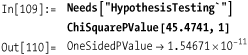
The second argument to ChiSquarePValue specifies the degrees of freedom of the distribution. In the solution example, we use 1 without explanation. The rule for computing the degrees of freedom for RC data is (numRows -1)(numCols -1).

In[111]:=  degreesOfFreedom[rc_List] := Times  @@ (Dimensions[rc] - 1)

In[112]:=  degreesOfFreedom[data]
Out[112]=  1

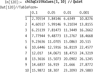
In the literature you will often find tables of critical values for various distributions relative to a significance level called alpha (α). For example, a common value for alpha is 0.05, which represents 95% confidence or (1 - α)* 100%. The critical value for a specified degree of freedom is the lower (or upper) bound for chiSquare in the solution that would give you the required confidence. Computing the critical value is the problem of finding a limit that gives the specified alpha as the area under the PDF for the distribution. We can compute these values efficiently using FindRoot and NIntegrate.

In[113]:=  chiSqUpperP[criticalValue_, df_] := With[{infinity = 1000}, NIntegrate[
              PDF[ChiSquareDistribution[df], x], {x, criticalValue, infinity}]]
           chiSqLowerP[criticalValue_, df_] := NIntegrate[
             PDF[ChiSquareDistribution[df], x], {x, 0, criticalValue}]
           criticalValueUpper[alpha_, df_] :=
            FindRoot[chiSqUpperP[c, df] == alpha, {c, 0.1}]
           criticalValueLower[alpha_, df_] :=
            FindRoot[chiSqLowerP[c, df] == alpha, {c, 0.1}]

The critical value for the experiment in the solution is

Our result was 45.47, so the result was well over the critical value. A result below the lower critical value is also acceptable, but clearly that does not apply to this experiment.

Given these functions, you can create your own tables of critical values like those in the NIST/SEMATECH e-Handbook of Statistical Methods website ( http://bit.ly/AbGvb ).

More information on using ChiSquare can be found in the NIST/SEMATECH e-Hand-book of Statistical Methods website (http://bit.ly/AbGvb).

A tutorial on the complete HypothesisTesting` package in Mathematica can be found in the documentation (HypothesisTesting/tutorial/HypothesisTesting).

You want to group data in separate lists based on a metric like Euclidean distance or Hamming distance. This problem arises in a wide variety of contexts, including market research, demographics, informatics, risk analysis, and so forth.

Use FindClusters with the default Euclidean distance function for numbers and vectors.

In[121]:=  FindClusters[{1, 100, 2, 101, 3, 102, 1000, 1010, 4, 1020, 7}]
Out[121]=  {{1, 2, 3, 4, 7}, {100, 101, 102}, {1000, 1010, 1020}}

When you use FindClusters with strings, this distance function is "edit distance" or the number of character changes to get from one string to another.

In[122]:=  FindClusters[DictionaryLookup[_~~ "ead" ~~ _]]
Out[122]=  {{beads, heads, leads, reads}, {beady, heady, Meade, Reade, ready}}

You can insist on a specific number of clusters.

In[123]:=  FindClusters[{1, 100, 2, 101, 3, 102, 1000, 1010, 4, 1020, 7}, 4]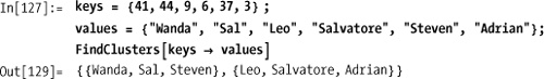
Out[123]=  {{1, 2, 3, 4}, {100, 101, 102}, {1000, 1010, 1020}, {7}}

If you need to cluster data by a key or criterion that is not part of the data, transform the data into the form {key1→data1, key2→data2, ...}. When FindClusters sees this format, it will cluster that data using the keys. For example, say you retrieve some data from a database with names and ages and you want to cluster names by age.

If you don’t want to lose the ages, you can use the following variation:

There is also a variation that is more convenient when the keys and values are in separate lists.

You can also handle the situation via a custom distance function, which is a more general solution since the function can use other metrics besides Euclidean distance.

Mathematica provides a variety of built-in distance functions that cater to different conceptions of closeness as well as different data types. For numbers, vectors, and higher-order tensors, you can use EuclideanDistance, SquaredEuclideanDistance, ManhattanDistance, ChessboardDistance, CanberraDistance, CosineDistance, CorrelationDistance, or BrayCurtisDistance. For example, CosineDistance (also known as angular distance) is often used with highly dimensional data. Here we generate a data set of 800 vectors of length 50. By design, the vectors are clumped into four groups by magnitude, so it should be of little surprise that FindClusters using default EuclideanDistance discovers four clusters.

In[131]:=  data =
             Join[RandomReal[{-10, -5}, {200, 50}], RandomReal[{-5, 0}, {200, 50}],
              RandomReal[{0, 1}, {200, 50}], RandomReal[{5, 10}, {200, 50}]];

In[132]:=  Length[FindClusters[data]]
Out[132]=  4

However, using CosineDistance, which is insensitive to vector length, only two clusters are found.

In[133]:=  Length[FindClusters[data, DistanceFunction -> CosineDistance]]
In[133]:=  2

For Boolean vectors, you can use MatchingDissimilarity, JaccardDissimilarity, RussellRaoDissimilarity, SokalSneathDissimilarity, RogersTanimotoDissimilarity, DiceDissimilarity, and YuleDissimilarity. Consider a problem that turns the game of 20 Questions on its head. I devised 20 questions in a somewhat haphazard fashion and then selected a bunch of nouns as they came into my head (Table 12-1). The idea here is to associate a Boolean vector with each noun based on how one might answer the questions in relation to the noun. Some of the questions are very subjective, and some don’t really apply to all nouns, but to stay in the domain of Boolean, I forced myself to choose either true or false.

The nouns I applied these questions to are

In[135]:= words = {"cat", "PC", "Java", "bird", "airplane", "Obama", "Mathematica",
             "Hillary Clinton", "weather", "time", "wind", "tunnel",
             "carpenter", "house", "red", "beer", "LSD", "Nintendo Wii",
             "John Lennon", "Paul McCartney", "Howard Stern", "mother", "Linux",
             "candle", "paper", "rock", "scissors", "steak", "broccoli"};

I’ll only show part of the data set (you can find it in the file 20Q.nb in the downloads from the book’s website).

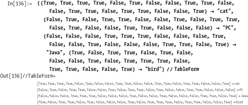
Assuming the full data set is stored in the variable data, we can see how FindClusters partitions the data using the various Boolean distance functions.

By transforming Boolean value to 0 and 1, you can see how EuclideanDistance and ManhattanDistance tend to create a larger number of clusters.

For strings, you can choose from EditDistance, DamerauLevenshteinDistance, and HammingDistance.

HammingDistance requires equal length strings, otherwise it will report an error. I added a preprocessing function that pads each string at the end with blanks to make each as long as the longest string in the list.

For advanced applications of FindCluster, you can tweak fine-grained aspects of the clustering algorithm via the Method option. Consult the FindClusters tutorial for detailed specifications of Method that provide for custom significance tests and linkage tests.

The tutorial for partitioning data into clusters (tutorial/PartitioningDatalntoClusters) is the essential resource for advanced features of FindClusters.

The Mathematica 7 function Gather is a special case of FindClusters: it groups identical elements, which is akin to clustering only when the distance is zero.

You want to visualize experimental data in a manner that effectively summarizes all the standard statistical measures.

The BoxWhiskerPlot is an excellent way to visually convey the essential statistics of one or more data sets.

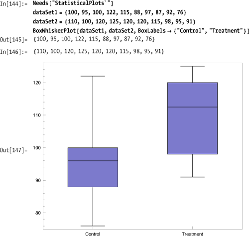
A box plot shows the minimum, maximum, median (black line), and middle quantile (box). There are options to change orientation (BoxOrientation), spacing (BoxExtraSpacing), styles (BoxLineStyle, BoxMedianStyle, BoxFillingStyle), and display of outliers (BoxOutliers, BoxOutlierMarkers). You can also show other quantiles using BoxQuantile.

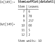
Other common statistical chart types include StemLeafPlot, ParetoPlot, QuantilePlot, and PairwiseScatterPlot.

A Pareto plot combines a bar chart of percentages of categories with a plot of cumulative percentages. It is often used in quality control applications for which the data might be defects for various products.

Quantile plots are used to visualize whether two data sets come from the same population. The closeness of fit to a straight line indicates the degree to which the data comes from the same population.

PairwiseScatterPlot plots each column of a matrix against each of the other columns. The diagonals will always be straight lines. The following plot of 2006, 2007, and 2008 Dow Jones Industrial Average (DJIA) data shows how 2006 and 2008 had nearly inverse trends, whereas 2007 deviated in the middle of the year from the 2008 data.

The tutorial StatisticalPlots/tutorial/StatisticalPlots in the documentation provides many examples for customizing these plots to your needs.

You need to generate random numbers, but you want to avoid the inevitable clustering that occurs using pseudorandom generators. This type of generator is sometimes called quasirandom.

Notice the clumping in this randomly generated list plot of 500 points.

The van der Corput sequence takes the digits of an integer in a given base b, and then reflects them about the decimal point. This maps the numbers from 1 to n into a set of numbers [0,1] in an even distribution, provided n is one less than a power of the base.

In[155]:=  corput[n_, b_] :=
             IntegerDigits[n, b].(b ^ Range[-Floor[Log[b, n] + 1], -1]);
           SetAttributes[corput, Listable]

The Halton sequence shows that a good way to distribute the values in n dimensions is to use the first n primes as the bases used with van der Corput.

As you can see, this gives far less clumpy distribution of points than RandomReal gives.

These quasirandom numbers are often used in simulations and Monte Carlo methods. One problem with these sequences is that they always give you the same set of numbers. One possibility is to perturb each number by a small random epsilon (e). This more or less preserves the even distribution provided the random perturbation is small.

An excellent reference is this Quasi-Monte Carlo Simulation website found at http://bit.ly/2vdGQs .

Interesting papers and Mathematica notebooks that explore quasirandomness can be found at James Propp’s University of Massachusetts Lowell website (http://bit.ly/7kC32).

You want to create a simulation as a means of developing a better understanding of the long-term behavior of a system governed by randomness.

One of the most well-known types of stochastic processes is the random walk. A random walk can occur in one-, two-, three-, or even higher dimensional space, but it is easiest to visualize in one or two dimensions. Here I show a random walk on a 2D lattice. A particle (or drunkard, if you prefer) starts at the origin {0,0} and can take a step east {0,1}, west {0,-1}, north {1,0} or south {-1,0}.

In[161]:=  latticeWalk2D[n_] := Module[{start = {0,0},
              east = {1, 0}, west = {-1, 0}, north = {0, 1}, south  = {0, -1}},
             NestList[# + RandomChoice[{east, west, north, south}] &, start, n]]

The walk is generated by specifying a number of steps and can be visualized using ListLinePlot or using arrows for each step, as I show in Out[163] below. Here I use SeedRandom only to make sure I always get the same walk no matter how many times this notebook is evaluated before going to press!

In[162]:=  SeedRandom[1004] ; walk  = latticeWalk2D[50]
Out[162]=  {{0, 0}, {-1, 0}, {0, 0}, {0, 1}, {0, 0}, {0, 1}, {-1, 1}, {-1, 2},
            {0, 2}, {-1, 2}, {-1, 1}, {-2, 1}, {-1, 1}, {-1, 2}, {0, 2}, {0, 1},
            {0, 2}, {-1, 2}, {-1, 1}, {-1, 0}, {-1, 1}, {-2, 1}, {-3, 1}, {-4, 1},
            {-4, 2}, {-5, 2}, {-5, 3}, {-6, 3}, {-6, 2}, {-5, 2}, {-6, 2}, {-6, 1},
            {-5, 1}, {-5, 0}, {-5, -1}, {-5, -2}, {-6, -2}, {-7, -2}, {-8, -2},
            {-9, -2}, {-10, -2}, {-10, -3}, {-10, -4}, {-11, -4}, {-10, -4},
            {-11, -4}, {-10, -4}, {-11, -4}, {-12, -4}, {-11, -4}, {-10, -4}}

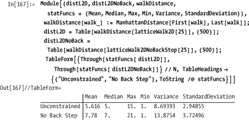
Some simulations contain constraints on what can happen at each step. For example, if you wanted a walk for which a back-step is disallowed, you could remember the previous step and remove its inverse from the population on the generation.

In[164]:=  latticeWalk2DNoBackStep[n_] :=
            Module[{start = {0, 0}, east = {1, 0}, west = {-1, 0},
              north = {0, 1}, south = {0, -1}, steps, last},
             steps = {east, west, north, south};
             (*Initialize last to a step not in the
              population so not to remove anything the first time.*)
             last = {1, 1};
             (*At each step the inverse (-last)
              is removed from possible steps using Complement.*)
             NestList[# + (last = RandomChoice[Complement[steps, {-last}]]) &,
              start, n]]

In[165]:=  SeedRandom[778]; walk = latticeWalk2DNoBackStep[25]
Out[165]=  {{0, 0}, {1, 0}, {2, 0}, {2, -1}, {3, -1}, {4, -1}, {5, -1}, {5, -2},
            {6, -2}, {6, -1}, {6, 0}, {5, 0}, {4, 0}, {4, 1}, {5, 1}, {5, 2}, {6, 2},
            {7, 2}, {7, 1}, {7, 0}, {8, 0}, {9, 0}, {9, 1}, {8, 1}, {8, 2}, {8, 3}}

Given a simulation, you will usually want to understand its behavior over many runs. One obvious metric is the distance from the origin. You might postulate, for example, that the average distance from the origin for latticeWalk2D will be less than latticeWalk2DNoBackStep. By running the simulation 500 times for each case and computing the mean, median, and other statistics, you can be more confident this intuition is correct. You can also see that the advantage seems to be only about two steps.

Simulation is also powerful as a tool for persuading someone of a truth that seems to defy intuition. A famous example is the Monty Hall problem. This problem is named after a U.S. game show called "Let’s Make a Deal," which was popular in the 1960s and ’70s and hosted by Monty Hall. A well-known statement of the problem was published in Parade magazine ("Ask Marilyn," Sept. 1990, 16):

For many people, the intuitive answer is that there is no advantage in switching because there is a 50/50 chance you have the car either way you go. There even seems to be a bias for not switching, based on the platitude "go with your first instincts." However, if you analyze the problem correctly (see the following analysis) there is a 2/3 probability of getting the car if you switch. But the analysis is subtle and apparently fails to convince even some very intelligent people, so perhaps a simulation is helpful. An advantage of creating the simulation is that it makes it clear just what you mean by this problem. Specifically, we are talking about the best decision over many trials for a problem where the initial choice of door is random, the placement of the car is random, and Monty always shows the door that contains a goat. In this simulation, we call sticking with your first choice strategyl and switching to the remaining door strategy2. The simulation is purposefully without any cute functional programming tricks so it is clear that at each step we are accurately following the rules of the game.

In[168]:=  (*randomPick is similar to RandomChoice except we want
            the position of the choice rather than the choice itself.*)
           randomPick[choices_List] :=
            Module[{}, RandomInteger[{1, Length[choices]}]]
           (*simulateStrat1VSStrat2 computes the winnings over a number
            of trials for strategy1 (stick) and strategy2 (switch).*)
           simulateStrat1VSStrat2[trials_Integer] :=
            Module[{GOAT = 0, CAR = 1, doors, firstPick, secondPick,
              winnings1 = 0, winnings2 = 0, doorsTemp, makePrizes},
             (*There are 3 possible initial game configurations. These
              can be generated using Permutations.*)
             SeedRandom[];
             Do[
              (*Randomly pick one of the
               three possible initial game configurations.*)
              doors = RandomSample[{GOAT, GOAT, CAR}];
              (*Contestant picks a door at random. Recall this
               is the position of the prize, not the prize itself.*)
              firstPick = randomPick[doors];
              (*Winnings of contestant who keeps first pick always*)
              winnings1 += doors[[firstPick]];
              (*Delete first pick from choices.*)
              doorsTemp = Drop[doors, {firstPick}];
              (*Delete goat from remaining; this is where Monty shows the goat.
                Here I use position to find a goat and, since there could be two,
                 I arbitrarily remove the first.*)
              doorsTemp = Drop[doorsTemp, Position[doorsTemp, GOAT][[1]]];
              (*Contestant following second
               strategy always switches to remaining prize.*)
              secondPick = doorsTemp[[1]];
              (*Winnings of contestant who switches*)
              winnings2 += secondPick,
              {trials}];
             {winnings1, winnings2}]

You can now simulate any number of games and compare the accumulated winnings over that many games. Here I show the results where the number of games varies from 10 to 100,000 in increments of powers of 10. Clearly strategy2, always switching, is the way to play the Monty Hall game.

   In[170]:=  Table[simulateStrat1VSStrat2[10^i], {i, 1, 5}] // TableForm
Out[170]//TableForm=
             4      6
             34     66
             304    696
             3345   6655
             33321 66679

The Monty Hall game analysis that leads to the correct conclusion is as follows: Consider the probability of not picking the car at the start of the game. Since there are 2 goats and 1 car, the probability of not picking a car is 2/3. Now consider what happens when Monty shows you a goat. In effect he tells you that IF you did not pick a car initially, THEN there is definitely a car behind the remaining door. We agreed that the probability of not having picked the car initially was 2/3, so now the probability of the car being behind the remaining door must be 2/3. The simulation we’re given shows this to be the case.

Computer Simulations with Mathematica: Explorations in Complex Physical and Biological by Richard J. Gaylord and Paul R. Wellin (Springer-Verlag TELOS) demonstrates a variety of simple simulations, but some of the examples need to be updated to Mathematica 6 and 7.

Chapter 14, contains an example of Monte Carlo simulation that is a very popular technique in finance and the physical sciences.

The Wolfram Demonstration Project ( http://bit.ly/40hsJD ) contains many small simulation problems that exploit Mathematica’s dynamic capabilities.