Time may change me But I can’t trace time I said that time may change me But I can’t trace time
—David Bowie, "Changes"
This chapter primarily focuses on the types of problems students and teachers will cover in college-level mathematics courses and how Mathematica can be used as a calculator (tool for getting an answer) and a teacher (tool for gaining insight into a mathematical problem). However, this focus was largely pragmatic and does not imply that Mathematica is limited to introductory calculus. Quite the contrary. Mathematica has been leading the charge among computer algebra systems since its inception, and with each new release the depth and breadth of its abilities in symbolic calculus improve. My goal in most of these recipes is to provide a starting point for the inexperienced user. Experts will probably find little that is new or highly original. This was a conscious choice based on space limitations. I am quite certain one could write a small cookbook by turning each recipe here into an entire chapter! Such is the depth of Mathematica’s abilities.
Most of the recipes in this chapter address what is commonly known
as infinitesimal or continuous calculus. These problems deal with limits
(11.1 Computing Limits), series (11.3 Using Power Series Representations), derivatives (11.4 Differentiating Functions), integrals (11.5 Integration), and differential equations (11.6 Solving Differential Equations). A common application of
calculus is finding minimums and maximums. Mathematica packages these
techniques into Minimize, Maximize,
and related functions (11.7 Solving Minima and Maxima Problems). When you use your
calculus skills to solve real engineering and physics problems, you are
bound to run smack into applications that involve vector calculus.
Mathematica has a package of functions specifically dedicated to vector
calculus, and we touch on some of this functionality in 11.8 Solving Vector Calculus Problems.
Although the calculus of continuous functions still plays a dominant role, discrete calculus is extremely important and has been garnering increasing attention lately due to research in such varied domains as string theory, probability theory, theory of algorithms, and combinatorics, to name a few. Mathematica 7 has enhanced its discrete calculus abilities. 11.9 Solving Problems Involving Sums and Products through 11.11 Generating Functions and Sequence Recognition help you start using these capabilities.
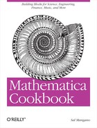
You want to determine the value of a function as a variable approaches a specific value, even if evaluating the function at that limit may give an indeterminate result.
The functions Sin[x]/x,
Sin[x^2]/x, and Sin[x]/x^2 each evaluate to the
indeterminate value 0/0 at x = 0; however, their limits as x approaches zero are quite definite and
different.

Plotting functions around the limiting value is often a good way to provide visual insight into the limiting value.

Here you can see that the last function has different
limits depending on whether one approaches the limit from the left or
the right. You can specify which limit you want using the option
Direction.
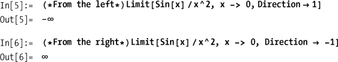
Mathematica supports a function Piecewise for composing a complex function
out of simpler functions using predicates to determine which of the
simpler functions apply.
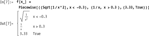

Clip, Sign, and
UnitStep are special cases of
built-in piecewise functions. Clip
constrains its input to a minimum and maximum value (default -1 and
+1). Sign gives -1 or 1 depending
on whether the input is negative or positive, and UnitStep is 0 for negative values and 1 for
values greater than or equal to zero.
You can differentiate and integrate piecewise functions, and you’ll get a piecewise function.

PiecewiseExpand can
take a nested piecewise function and return a single function. You can
use this to show that Min, Max, and
Abs are also special cases of
piecewise functions.

The Mathematica function Series will generate the series expansion of
a function about a point to a specified order. It produces a SeriesObject, which Mathematica will display
as a traditional series expansion.
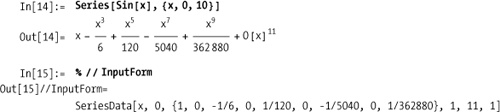
You use Normal to create a
regular Mathematica expression. Here I also use Evaluate because I am defining a function
and want Normal to evaluate
immediately even though the function is defined using SetDelayed (:=). Equivalently, you can use
Set (=) to define the function
without Evaluate.
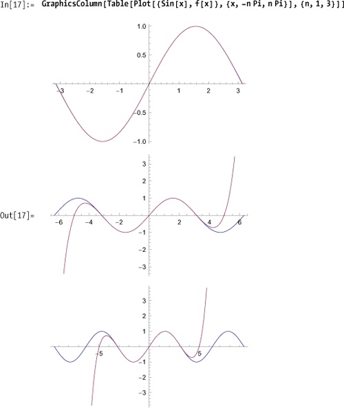
In[16]:= f[x_] := Evaluate[Normal[Series[Sin[x], {x, 0, 10}]]]You visualize the accuracy of the series approximation by plotting over successively larger intervals. As expected, this series approximation begins to diverge as you move away from the origin.


You want to compute derivatives or partial derivatives of functions in symbolic form. You may do this as a means of creating new functions or as a means of teaching the concepts that underlie differentiation.
Mathematica allows you to enter derivatives in input form as
D[f[x], x] or in standard form as
∂x
        f[x]
.
In[20]:= D[Sin[x],x]
Out[20]= Cos[x]

In[21]:= ∂xSin[x]
Out[21]= Cos[x]
Higher-order derivatives are specified as D[f[x],{x,n}] where n
is 2 for the second derivative, 3 for the third, and so on. In
standard form, the second derivative can be entered as ∂{x,2} f[x].
In[22]:= D[Sin[x], {x, 2}]
Out[22]= -Sin[x]
Partial derivatives are easily accommodated as well using several equivalent notations.
In[23]:= D[Sin[x] Sin[y], {x, 1}]
Out[23]= Cos[x] Sin[y]

In[24]:= D[Sin[x] Sin[y], x, x, y]
Out[24]= -Cos[y] Sin[x]

In[25]:= D[Sin[x] Sin[y], {x, 2}, {y, 1}]
Out[25]= -Cos[y] Sin[x]
Mathematica also recognizes prime notation, but this notation is more commonly used in Mathematica when entering a differential equation. See the sidebar Mathematica’s Representation of Differentiation for some important subtleties.
In[26]:= {Sin'[x], Sin''[x]}
Out[26]= {Cos[x], -Sin[x]}
You can use D along with
Solve to differentiate implicit
functions. Simply use D as usual
and use Solve to find the solution
in terms of y'[x].

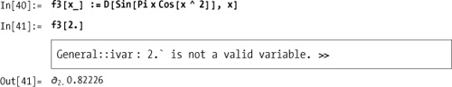
There are cases where you may want to use the D to synthesize a function on the fly. In
this case, use Set (=) to perform
the differentiation operation immediately or use Evaluate with SetDelayed (:=).
In[37]:= f1[x_] = D[Sin[Pi x Cos[x ^ 2]], x];

In[38]:= f2[x_] := Evaluate[D[Sin[Pi x Cos[x ^ 2]], x]]

In[39]:= {f1[2.], f2[2.]}

Out[39]= {-9.65614, -9.65614}
If you forget to do so, you will get an error when you call the function with a literal value.
Mathematica’s Representation of Differentiation
More importantly, the prime notation is not synonymous
with D[] but rather with a
differential operator of the form Derivative[n]. The operator form clarifies
ambiguities that would result from using it with functions of more
than one variable. Think of Derivative[n1,
n2, ...] as an operator that acts on a function to produce
the specific derivative. The number of n’s
should not exceed the number of variables of the function since each
n is associated with the nth derivative of the
corresponding variable. Some examples should help clarify.
First derivative with respect to x:
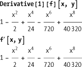
First derivative with respect to x, then y:
Derivative[1,1][f][x,y]
f(1,1) [x,y]
First derivative with respect to x, then second derivative with respect to y:
Derivative[1, 2][f][x, y]
f(1,2) [x,y]
For the most part, you should work with D[] directly, but keep the operator
notation in the back of your mind because it is how Mathematica
represents derivatives internally.
D[f[x, y], x, y] // FullForm
Derivative[1, 1][f][x, y]

Derivative[1, 1][f][x, y]
f(1,1)[x,y]
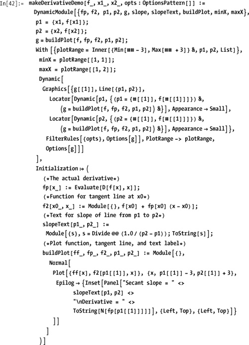
Many students will use Mathematica to check the answers to their calculus homework, but Mathematica is also useful for generating demonstrations of the fundamental concepts underlying differentiation. For example, the derivative of a function at a point is the slope of the tangent to the function at that point. Further, given two points, the slope of the secant drawn between these points approaches the derivative as the points approach each other along the curve. The following function uses Mathematica’s dynamic features to generate presentations of this fact using any function and starting points as input.

You want to solve problems that involve indefinite or definite integrals using symbolic integration.
Use Integrate or ∫ to compute
single, double, or higher-order integrations. Indefinite integrals
specify an expression and the variables of integration.
In[44]:= Integrate[1/x, x]
Out[44]= Log[x]
Definite integrals provide the minimum and maximum limits, which can be constants or expressions.
The minimum and maximum limits can be -Infinity or Infinity.
In[48]:= Integrate[1 /(x^3 + x^2), {x, 1, Infinity}]
Out[48]= 1 - Log[2]Integrate will easily handle
most integration problems you are likely to encounter in school,
engineering, and science.

Double and higher-order integrals are computed with a single
Integrate function by adding
multiple integration variables. However, if you use the traditional
integration notation, you will use multiple integral symbols.

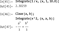
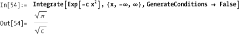
Some integrations may return with conditionals and assumptions due to convergence issues. You can eliminate these by providing your own assumptions.

You also do this using GenerateConditions → False.
You can also get piecewise functions as a result of Integrate.

When Integrate is unable to
solve the integration, it will return the unevaluated integral in
symbolic form.

Applications of integration are numerous, and it would be
impossible to provide even a small representative set of examples
here. Rather, I will provide examples that emphasize how Integrate can be combined with other
Mathematica functions in non-obvious ways.
A simple application is a function to compute the area between
two arbitrary curves given two points. When you create functions that
embed Integrate, you often want to
allow options to pass through to increase generality.

This would generate a huge messy conditional if not for the
ability to pass assumptions about the arbitrary bounds a and b.
Create a table of volumes of hyperspheres. Here Boole maps True to 1 and False to 0. Note that the list of
integration limits must be converted to a sequence using Apply (@@). By the
way, this is a very expensive way to calculate volume of a
hypersphere, but it does illustrates how to parameterize the order of
integration. Search for hyperspheres on Wikipedia or Wolfram’s
MathWorld to find a more practical formula.

You can combine Integrate
with differentiation to create a general function to compute the
length of a curve between two points.
In[61]:= Clear[lengthOfCurve]

In[62]:= lengthOfCurve[expr_, var_, a_, b_, opts : OptionsPattern[]] :=
          Integrate[Sqrt[1 + D[expr, var] ^ 2], {var, a, b},
           Sequence @@ FilterRules[{opts}, Options[Integrate]]]
Or, you can compute the length of the hypotenuse of a right triangle.
Verify the formula for the circumference of a circle given its radius by taking twice the arc length of a semicircle.
Here is a purely symbolic solution with assumptions to simplify results.

You have a model of a system described by a differential equation and you want to solve that equation symbolically. Two related problems are getting the equation in a form Mathematica expects and getting the solution in the form you expect.
An undergraduate student of engineering or physics will commonly need to solve differential equations that model simple systems. A common problem is an undamped oscillator composed of a mass hanging from a spring. The problem may appear in a textbook as
In[66]:= m y'' + k y = 0This says that the force (mass × acceleration) is balanced by
the force of the spring, as given by Hooke’s law, where k is the spring constant. The key to solving
this equation in Mathematica using DSolve is to make the equation more
explicit. Specifically, the equation omits the time variable. You must
also replace the = symbol with == and tell Mathematica what equation
we are solving for and what are the variables.

The solution is given as a replacement rule, and since the
equation is a second order, two constants, C[1] and C[2], are introduced. You can provide
initial conditions to eliminate the constants. In this case, you can
also render the solution in its customary form by replacing Sqrt[k]/Sqrt[m] by the angular frequency
ω.

The solutions provided by DSolve are not automatically simplified, and
you often will want to use Simplify
or FullSimplify to postprocess them
into a more mathematically friendly form. This is especially relevant
when comparing the answer DSolve finds with answers provided in a
typical textbook. Consider this problem adapted from
Advanced Engineering Mathematics by Erwin
Kreyszig (John Wiley). Here you want to find the solution to a
differential equation describing the speed of a fluid flowing out of
an opening in a container.

Given the physics of the problem, it should be clear we want the first solution (the second solution has the height increasing with time).
Although this has simplified the result somewhat, it is a much more complicated solution than the one provided by Kreyszig, which is

Did DSolve give the wrong
result? A common mistake when using Mathematica is to prematurely
substitute specific constants as I did above. It is often advisable to
solve equations entirely in symbolic form and substitute constants
later.

Although this did not get us all the way to the form of the
book’s solution, you are more likely to see the final transformation
that will demonstrate that DSolve
was correct. It hinges on noticing that 1/4 is the same as (-1/2)*(-1/2).
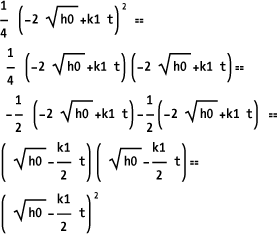
Substituting h0 and
kl with the constants shows that
Mathematica did get the correct solution. Alternatively, you can ask
Mathematica to prove its solution is equal to the book’s solution by
using Resolve and ForAll. The only problem here is that
Mathematica does not show its work!

You want to find the minimum or maximum values of a function. You may need to find these extremes subject to constraints or for numbers in a specific domain (e.g., integers).
Although there are standard techniques used in calculus for
finding extrema, Mathematica provides the specific functions Minimize and Maximize, which provide a great deal of
power.

For many applications of minimization or maximization, you are interested in the extreme value within a specific interval.
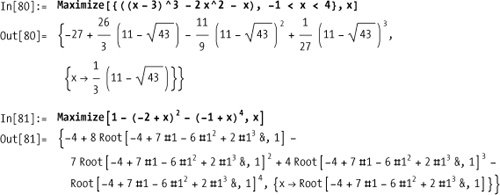
I restrict this discussion to Maximize for simplicity, but everything here
applies to Minimize as well. If you
are interested in displaying the result of Maximize, you will want to force the result
to numerical form, as we did in the solution. Maximize will keep the result in exact form
if it is given input in exact form. For polynomials, this typically
means the result will be expressed in terms of radicals or Root objects. A Root[f,k] object represents the kth solution
to a polynomial equation f[x] ==
0.
Sometimes you want to find solutions for integer values
only. You can constrain Maximize to
the integers in one of two ways. You might recognize this problem as
an instance of a knapsack problem where you are optimizing the value
of the knapsack (item1 has value 8, item2 11, and so on) subject to
size constraint of 14 where item1 has size 5 and so on.

A more convenient notation when all variables are integer is to
specify the domain as the third argument to Maximize.

Maximize seeks a global
maximum, whereas an alternative function, FindMaximum, seeks a local maximum (there is
also FindMinimum for local
minimums). FindMaximum allows you
to specify a starting point for the search, but otherwise has a very
similar form to Maximize. The
following program demonstrates the difference between Maximize and FindMaximum. The advantage of FindMaximum is that it does not require the
objective function to be differentiable.

You want to find solutions to problems within vector fields. Such problems arise in mechanics, electromagnetic theory, and fluid dynamics.
Simple vector calculus problems can be solved in terms of the
calculus primitives discussed in this chapter’s recipes along with
vector functions like Dot and
Cross. For example, line integrals
are commonly used to calculate work performed when moving a particle
along a path in a vector field. Here F is the vector equation of the field,
f is the equation of the path
through the field, var is the
parameter of f, and a and b
are the start and end points of the path.

Another common operation in vector calculus is the
surface integral over scalar functions and vector fields. Surface
integrals are the 2D analog of line integrals. One way to think of the
scalar surface integral is to imagine a surface f made of a material whose density varies as
described by a second function g.
The surface integral of f over
g is then the mass per unit
thickness.
In[93]:= surfacelntegralScalar[g_, f_, {v1_, v1a_, v1b_}, {v2_, v2a_, v2b_}] :=
          Integrate[g[f[v1, v2]] Norm[Cross[D[f[v1, v2], v1], D[f[v1, v2], v2]]],
           {v1, v1a, v1b}, {v2, v2a, v2b}]
For example, consider the surface fl, which is a half sphere over the interval
{ ϕ , 0,
Pi/2} and {
θ , 0, 2 Pi}, and compute the surface integral
given a density function given by (x^2 + y^2)
z.

If we use a constant function (uniform density), we get the surface area of the half sphere as expected (surface area of an entire sphere is 4 πr2).
In[97]:= g2[{x_, y_, z_}] := 1
         surfaceIntegralScalar[g2, f1, {ϕ, 0, Pi/2}, {θ, 0, 2 Pi}]
Out[98]= 2 π
For a vector field, there is a similar equation using Dot in place of scalar multiplication by the
norm. The traditional way to visualize the vector surface interval is
to consider a fluid flowing through a surface where there is a vector
function F describing the velocity
of the fluid at various points on the surface. The surface integral is
then the flux, or the quantity of fluid flowing
through the surface in unit time.
In[99]:= surfaceIntegralVector[F_, f_, {v1_, v1a_, v1b_}, {v2_, v2a_, v2b_}] :=
          Integrate[Dot[F[f[v1, v2]], Cross[D[f[v1, v2], v1], D[f[v1, v2], v2]]],
           {v1, v1a, v1b}, {v2, v2a, v2b}]
Here is the solution to the flux described by {3 y, -z, x^2} through a surface described
parametrically as {s t, s + t, (s^2 -
t^2)/2}.
In[100]:= f[s_, t_] := {s t, s + t, (s^2 - t^2) /2}
          F[{x_, y_, z_}] := {3 y, -z, x^2}
          surfaceIntegralVector[F, f, {s, 0, 1}, {t, 0, 3}]
Out[102]= -15
A standard result from electrostatics is that the net flux out of a unit sphere, for a field that is everywhere normal, is zero. We can verify this as follows:
In[103]:= F2[{x_, y_, z_}] := {1, 1, 1}/(x^2 + y^2 + z^2)

In[104]:= f2[θ_, ϕ_] := {Sin[ϕ] Cos[θ], Sin[ϕ] Sin[θ], Cos[ϕ]}

In[105]:= surfaceIntegralVector[F2, f2, {θ, 0, 2 Pi}, {ϕ, 0, Pi}]

Out[105]= 0
The solution shows how the calculus primitives and other
Mathematica functions can be used to build up higher-order vector
calculus solutions. However, if you are interested in solving problems
in vector calculus, the package VectorAnalysis` is definitely worth a look.
Be forewarned that you might be in for a bit of a learning curve with
this particular package, but it offers a lot of functionality. An
important feature of the package is that it simplifies working in
different coordinate systems. Before you can make effective use of
VectorAnalysis`, you need to
understand how coordinate systems are used and which coordinate system
is appropriate to your problem.
In[106]:= Needs["VectorAnalysis`"]

In[107]:= CoordinateSystem
Out[107]= Cartesian

In[108]:= SetCoordinates[Spherical]
Out[108]= Spherical[Rr, Ttheta, Pphi]

In[109]:= CoordinateSystem
Out[109]= Spherical
When you use VectorAnalysis`,
you will typically want to use functions in that package in place of
some standard Mathematica functions such as Dot and Cross. This is because the alternatives
DotProduct and CrossProduct respect the current coordinate
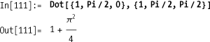
system. For example, if the current coordinate system is Spherical, you expect the following DotProduct to be zero because the vectors
are orthogonal in spherical coordinates.
In[110]:= DotProduct[{1, Pi/2, 0}, {1, Pi/2, Pi/2}]
Out[110]= 0
In contrast, Dot and
Cross always assume Cartesian
coordinates.
Some of the most important vector calculus operations are
Div (divergence), Grad (gradient), Curl, and the Laplacian. Although it would make a nice
exercise to implement these from the calculus primitives, as I did for
line and surface integrals, there is no need if you use the VectorAnalysis` package. These operations
use the default coordinate system, or you can specify a specific
coordinate system as a separate argument.
The divergence represents the instantaneous outflow of a vector field at each point.

The curl of a vector field represents the amount of rotation.

By definition, the divergence of the curl must be zero since the curl has no net outflow.
In[114]:= SetCoordinates[Cartesian[x, y, z]];
          Div[Curl[{1, 1, 1} / (x^2 + y^2 + z^2)]]
Out[115]= 0
The gradient of a function f
is a vector-valued function that indicates the direction in which
f is increasing most rapidly. If
you were climbing a hill, you would move in the direction of the
gradient at each point to reach the top (strictly speaking the
gradient would only be guaranteed to be directing you to a local
peak). You can visualize the meaning of the gradient by using VectorPlot. I restrict the result to 2D for
easier visualization.

You want to solve problems in discrete calculus that are expressed in terms of sums or products.
Mathematica can handle infinite sums and products with ease, provided, of course, they converge.

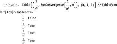
If sums or products don’t converge, Mathematica will let
you know by emitting an error. You can test for convergence without
evaluating the sum using SumConvergence.

As with Integrate, Sum can specify multiple summation
variables. In traditional form these sums are rendered as a multiple
summation, but keep in mind that these are entered as Sum[expr,{n,nmin,nmax},{m,mmin,mmaz}] rather
than Sum[Sum[expr,
{n,nmin,nmax}],{m,mmin,mmaz}].
This double summation has a surprisingly simply solution.
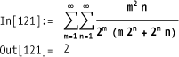
This is a very famous sum attributed to Srinivasa Ramanujan, one of India’s greatest mathematical geniuses. You might think that Mathematica is just doing some simple pattern matching to recognize this result; however, substitute for any of the magic constants in this formula, and Mathematica will handle it just as well (but don’t expect the answer to be as pretty).
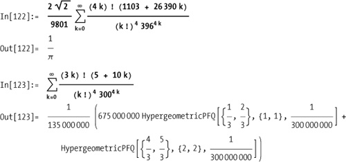
Here is a very pretty formula for π that combines an infinite sum and an infinite product.

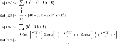
As of version 7, Mathematica can handle indefinite sums and
products. Mathematica will seek to eliminate the sum if possible. For
example, the sum over k of a
polynomial is another polynomial that can be expressed in terms of
k, and products over polynomials
will invariably reduce to some expression involving Gamma.
The Z-transform is an important infinite sum used in signal
processing. It is defined as Sum[f[n]
z^-n,{n, 0, Infinity}], but is directly supported using
ZTransform.

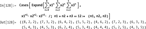
Here is an unconventional application for Sum, but one that is sometimes used in
discrete math to introduce the idea of a generating function. You can
use Sum to construct a generating
function for solutions to problems like n1+n2+n3 == 12 subject to nl >= 4, n2 >= 2, and 5 >= n3 >= 2. Each Sum is constructed
from the smallest number the associated variable can take to the
largest, by considering the smallest the other variables can take. For
example, xl must be at least 4 but
can’t be greater than 12-2-2 = 8, since n2 and n3
must each be at least 2. Here we use Expand to generate the polynomial
and Cases to find the exponents
that sum to 12, thus giving all solutions.
If you only care about the number of solutions, it would fall out of the coefficient of x12 in the expansion of this polynomial.

See 11.11 Generating Functions and Sequence Recognition for more information on generating functions in Mathematica.
Readers who are interested in gaining insight into the algorithms that underlie Mathematica’s amazing feats with infinite sums should read A=B by Marko Petkovsek, Herbert S. Wilf, and Doron Zeilberger (A K Peters), which is available online at http://bit.ly/1LJiwe .
You want to solve problems that arise in discrete systems such as finance, actuarial science, dynamical systems, and numerical analysis. Many such problems can be modeled as recurrence relations, also known as difference equations.
RSolve is used to
solve difference equations. A simple problem where RSolve applies is in mortgage calculations.
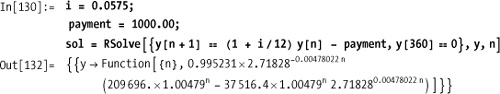
Suppose you want to derive a function for the outstanding principal
over the life of a loan. Let’s say the yearly interest rate is 5.75%,
the monthly payment is $1,000.00, and the term is 30 years. This loan
can be described as the following difference equation. Here the
constraint y[360] == 0 arises from
the condition that the last payment is zero (I am using y[0] as the origin).
From this we can figure out the initial principal or the payoff at any given month:
In[133]:= y[0] /. sol[[1]]
Out[133]= 171358.
After 60 months, or 5 years, very little has been paid off, which is quite depressing but a fact of life.
In[134]:= y[0] - y[60] /. sol[[1]]
Out[134]= 12402.6Setting up a difference equation is often a matter of solving
the problem by hand for small values of n and
then detecting the relationship between successive values. Consider
the Towers of Hanoi puzzle. A one-disk problem is solved in one move
(T[1] = 1), a two-disk problem is
solved in three moves (T[2] = 3),
and three-disk problem is solved in seven moves (T[3] = 7). It follows then that T[n] = 2 T[n-1] + 1.
A seemingly innocent difference equation can result in a solution involving complex numbers. This is a second-order equation, so two initial values are required to get an exact solution with no arbitrary constants.

Note that like DSolve,
RSolve does not try to simplify the result. It is advisable
to try to simplify it; in this case, you see that complex numbers
disappear, and the result is in terms of trigonometric functions,
which you may not have expected.
As with DSolve, if you do not
provide initial conditions, you will get solutions involving arbitrary
constants of the form C[N].
These solutions were found in terms of pure functions because we
asked for the solution in terms of a, but you can change the form of the second
argument to a[n] to get the
solution in that form.
You can evaluate this solution for specific n and C[1] using ReplaceAll (//.).
You want Mathematica to generate a function associated with a particular sequence or to infer a function that will produce the sequence for successive integers.
Use FindGeneratingFunction to derive the
generating function for a sequence. Recall that the power series of a
generating function encodes the sequence in its coefficients.

Use FindSequenceFunction to
find an expression that maps the integers to the specified
sequence.
In[143]:= s = FindSequenceFunction[{1, 4, 9, 16, 25, 36, 49, 64, 81, 100}, n]
Out[143]= n2

In[144]:= Table[s, {n, 1, 12}]
Out[144]= {1, 4, 9, 16, 25, 36, 49, 64, 81, 100, 121, 144}
FindSequenceFunction can deal
with sequences that are not strictly increasing and with noninteger
sequences.

You can synthesize a generating function from an expression
using GeneratingFunction.

And recover the sequence to the Nth term using the following
expression:
In[148]:= With[{N=12},
           1/Table[SeriesCoefficient[Simplify[Series[g, {x, 0, N}]], n], {n, 1, N}]]
Out[148]= {2, 6, 24, 120, 720, 5040, 40320, 362880,
           3628800, 39916800, 479001600, 6227020800}
For the nonexpert, a very approachable book on generating functions is Generatingfunctionology by Herbert S. Wilf (A K Peters). An online version can be found at http://bit.ly/3bkssK .