Many books on Mathematica tout its capabilities as a multiparadigm language. Although it’s true that Mathematica supports procedural, recursive, rule-based, functional, and even object-oriented styles (to some degree), I believe it is the functional and rule-based styles that are most important to master. Some gurus may go a step further and say that if you do not master the functional style then you are not really programming in Mathematica and your programs will have a far greater chance of being inefficient and clumsy. I won’t be so dogmatic, but until you are an expert it’s best to stick with an approach that many Mathematica experts prefer. A practical reason to learn the functional style is that most of the recipes in this book use either functional or rule-based styles and sometimes mixtures of both. This chapter is intended as a kind of decoder key for readers who want to master the functional style and get a deeper understanding of the solutions throughout this book. There are also a few recipes at the end of the chapter that are not about functional programming proper, but rather techniques specific to Mathematica that allow you to create flexible functions. These techniques are also used throughout later recipes in the book.

The hallmark of the functional style is, of course, functions. Every high-level programming language has functions, but what makes a language functional is that functions are first-class entities (however, see the sidebar What Is a Functional Programming Language and How Functional Is Mathematica? for more subtle points). This means you can write higher-order functions that take other functions as arguments and return functions as values. Another important feature of functional languages is that they provide a syntactic method of whipping up anonymous functions on the fly. These nameless functions are often referred to as "lambda functions," although Mathematica calls them pure functions.

Unless you are already a convert to functional programming, why a functional approach is considered superior may not be obvious to you. A general consensus among software developers is that given two correct solutions to a problem, the simpler solution is the superior one. Simplicity is sometimes difficult to define, but one metric has to do with the length of the solution in lines of code. You will find, almost without exception, that a high-quality functional solution will be more concise than a high-quality procedural solution. This stems partly from the fact that looping constructs disappear (become implicit) in a functional solution. In a procedural program, code must express the loop, which also introduces auxiliary index variables.

Functional programs are often faster, but there are probably exceptions. Ignoring the fact that Mathematica has a built-in function, Total, for a moment, let’s contrast a procedural and functional program to sum an array of 100,000 random values.

In[1]:= array = RandomReal[{-1, 1}, 100000];

In[2]:= (*Procedural solution using For loop*)
        (sum = 0 ;
          Do[sum += array[[i]], {i, 1, Length[array]}];
          sum) // Timing
Out[2]= {0.21406, 90.6229}

In[3]:= (*Functional solution using Fold*)
        Fold[Plus, 0, array] // Timing
Out[3]= {0.008291, 90.6229}

As you can see, the functional solution was about an order of magnitude faster. Clearly the functional solution is shorter, so that is an added bonus. Of course, one of the tricks to creating the shortest and the fastest programs is exploiting special functions when they exist. In this case, Total is the way to go!

In[4]:= Total[array] // Timing
Out[4]= {0.000193, 90.6229}

If you come from a procedural background, you may find that style more comfortable. However, when you begin to write more complex code, the procedural style begins to be a liability from a complexity and performance point of view. This is not just a case of shorter being sweeter. In a very large program, it is common to introduce a large number of index and scratch variables when programming procedurally. Every variable you introduce becomes a variable whose meaning must be tracked. I wish I had a dollar for every bug caused by a change to code that used index variable i when j was intended! It should come as no surprise that eliminating these scratch variables will result in code that is much faster. In fact, in a typical procedural language like C, it is only through the efforts of a complex optimizing compiler that these variables disappear into machine registers so that maximum speed is obtained. In an interpreted language like Mathematica, these variables are not optimized away and, hence, incur a significant overhead each time they appear. By adopting a functional approach, you get almost the equivalent of optimized machine code with the pleasure of interactive development.

There are a lot more theoretical reasons for adopting a functional approach. Some involve the ability to prove programs correct or the ability to introduce concurrency. I will not make those arguments here because they usually have only marginal value for practical, everyday development and they hinge on a language being purer than Mathematica. Readers who have interest in learning more should refer to some of the excellent resources listed in the See Also.

Many functional programming languages share core primitive functions that act as the building blocks of more sophisticated functions and algorithms. The names of these primitives vary from language to language, and each language provides its own twists. However, when you learn the set of primitives of one functional language, you will have an easier time reading and porting code to other functional languages.

FoldList [f,x,
 {a1, a2, a3, ...}]

Note

In the Mathematica documentation, you will see the verb apply (in its various tenses) used in at least two senses. One is in the technical sense of the function Apply[f,expr] (i.e., change the head of expr to f) and the other in the sense of invoking a function on one or more arguments (as in "applied" in the definition of Nest[], "gives an expression with f applied n times to expr"). Clearly, changing the head of the expression n times would be no different from changing it once, so it should be unambiguous in most cases. See 2.1 Mapping Functions with More Than One Argument for syntax variations of the latter sense of function application.

There are other important Mathematica functions related to functional programming, but you should commit to memory the functions in Table 2-1, because they arise repeatedly. You should especially get used to the operator notations for Map (/@) and Apply (@@) because they arise frequently (not only in this book but in others and in sample code you will find online). If you are unfamiliar with these functions, it is worthwhile to experiment a bit. One important exercise is to use each function with a symbol that is not defined and a list of varying structure so you can see the effects from a structural point of view. For example, pay close attention to the difference between /@ and @@@. Each iterates the function across the list, but the results are quite different.

Note

In this code, zz is purposefully undefined so you can visualize the effect of the operators. The ability of Mathematica to handle undefined symbols without throwing errors is both a source of power and a source of frustration to the uninitiated.

 In[5]:= zz /@  {1, {1}, {1, 2}}
 Out[5]= {zz[1], zz[{1}], zz[{1, 2}]}
 In[6]:= zz @@ {1, {1}, {1, 2}}
 Out[6]= zz[1, {1}, {1, 2}]
 In[7]:= zz @@@ {1, {1}, {1, 2}}
 Out[7]= {1, zz[1], zz[1, 2]}
 In[8]:= Fold[zz, 0, {1, {1}, {1, 2}}]
 Out[8]= zz[zz[zz[0, 1], {1}], {1, 2}]
 In[9]:= FoldList[zz, 0, {1, {1}, {1,2}}]
 Out[9]= {0, zz[0, 1], zz[zz[0, 1], {1}],
          zz[zz[zz[0, 1], {1}], {1, 2}]}
In[10]:= Nest[zz, {1, {1}, {1, 2}},3]
Out[10]= zz[zz[zz[{1, {1}, {1, 2}}]]]
In[11]:= NestList[zz, {1, {1}, {1, 2}},3]
Out[11]= {{1, {1}, {1, 2}}, zz[{1, {1}, {1, 2}}],
          zz[zz[{1, {1}, {1, 2}}]],
          zz[zz[zz[{1, {1}, {1, 2}}]]]}

Mathematica has a flexible facility for associating symbols and their definitions. Most of the time you need not be concerned with these low-level details, but some advanced Mathematica techniques discussed in this chapter and elsewhere in the book require you to have some basic understanding. When you define functions of the form f[args] := definition or f[args] = definition you create downvalues for the symbol f. You can inspect these values using the function DownValues[f].

The results are shown as a list of patterns in held form (see 4.8 Preventing Evaluation Until Replace Is Complete). The order of the definitions returned by DownValues is the order in which Mathematica will search for a matching pattern when it needs to evaluate an expression containing f. Mathematica has a general rule of ordering more specific definitions before more general ones; when there are ties, it uses the order in which the user typed them. In rare cases, you may need to redefine the ordering by assigning a new order to DownValues[f].

There are some situations in which you would like to give new meaning to functions native to Mathematica. These situations arise when you introduce new types of objects. For example, imagine Mathematica did not already have a package that supported quaternions (a kind of noncommutative generalization of complex numbers) and you wanted to develop your own. Clearly you would want to use standard mathematical notation, but this would amount to defining new downvalues for the built-in Mathematica functions Plus, Times, etc.

Unprotect[Plus,Times]
Plus[quaternion[a1_,b1_,c1_,d1_], quaternion[a2_,b2_,c2_,d2_]] := ...
Times[quaternion[a1_,b1_,c1_,d1_], quaternion[a2_,b2_,c2_,d2_]] := ...
Protect[Plus,Times]

If quaternion math were very common, this might be a valid approach. However, Mathematica provides a convenient way to associate the definitions of these operations with the quaternion rather than with the operations. These associations are called UpValues, and there are two syntax variations for defining them. The first uses operations called UpSet (^=) and UpSetDelayed (^:=), which are analogous to Set (=) and SetDelayed (:=) but create upvalues rather than downvalues.

Plus[quaternion[a1_,b1_,c1_,d1_], quaternion[a2_,b2_,c2_,d2_]] ^:=  ...
Times[quaternion[a1_,b1_,c1_,d1_], quaternion[a2_,b2_,c2_,d2_]] ^:= ...

The alternate syntax is a bit more verbose but is useful in situations in which the symbol the upvalue should be associated with is ambiguous. For example, imagine you want to define addition of a complex number and a quaternion. You can use TagSet or TagSetDelayed to indicate that the operation is an upvalue for quaternion rather than Complex.

quaternion /: Plus[Complex[r_, im_], quaternion[a1_,b1_,c1_,d1_]] := ...
quaternion /: Times[Complex[r_, im_], quaternion[a1_,b1_,c1_,d1_]] := ...

Upvalues solve two problems. First, they eliminate the need to unprotect native Mathematica symbols. Second, they avoid bogging down Mathematica by forcing it to consider custom definitions every time it encounters common functions like Plus and Times. (Mathematica aways uses custom definitions before built-in ones.) By associating the operations with the new types (in this case quaternion), Mathematica need only consider these operations in expression where quaternion appears. If both upvalues and downvalues are present, upvalues have precedence, but this is something you should avoid.

Mathematica will modulate the behavior of functions based on a set of predefined attributes, which users should already be familiar with as those often required to achieve proper results in users’ own functions. The functions Attributes[f], SetAttributes[f,attr], and ClearAttributes[f,attr] are used to query, set, and clear attributes from functions. In the following subsections, I’ll review the most important attributes. Refer to the Mathematica documentation for attributes to review the complete list.

Note

Attributes must be assigned to symbols before functions are defined for the symbols.

An excellent animated introduction to the core Mathematica functions can be found at http://bit.ly/3cuB4B.

See guide/FunctionalProgramming in the documentation for an overview of Mathematica’s functional programming primitives.

A classic paper on the benefits of functional programming is Why Functional Programming Matters by John Hughes ( http://bit.ly/4mRBYO ).

Another classic is A Tutorial on the Universality and Expressiveness of Fold by Graham Hutton (PDF available at http://bit.ly/ZYDiH ).

Further discussion of upvalues and downvalues can be found at tutorial/TheStandardEvaluationProcedure and tutorial/AssociatingDefinitionsWithDifferentSymbols in the documentation.

You need to map a function over a list containing sublists whose values are arguments to the function.

Use a Map-Apply idiom. A very simple example of this problem is when you want to sum the sublists.

In[18]:= Map[(Apply[Plus, #]) &, {{1,2,3}, {4,5,6,7,8}, {9,10,11,12}}]
Out[18]= {6, 30, 42}

This can be abbreviated to:

In[19]:= Plus @@ # & /@ {{1, 2, 3}, {4, 5, 6, 7, 8}, {9, 10, 11, 12}}
Out[19]= {6, 30, 42}

Although the solution seems very simple, this problem arises quite frequently in more complicated guises, and you should learn to recognize it by studying some of the following more interesting examples.

Consider a structure representing an order for some product with the form order[sku, qty,price]. Now imagine you have a list of such orders along with a function for computing the total cost of an order. Given a list of orders, you want to produce a list of their costs. The situation is a bit tricky because our function does not care about the sku, and rather than a list of lists we have a list of order[]. Even with these differences you still have the same basic problem. Recall that Apply does not necessarily require an expression whose head is List; it will work just as well with any head, such as order. Also, using compOrderTotCost we can easily preprocess each order to extract just the elements needed.

In[20]:= compOrderTotCost[qty_, price_] := qty * price
         Map[(Apply[compOrderTotCost, Rest[#]]) &, {order["sku1", 10, 4.98],
           order["sku2",  1, 17.99], order["sku3", 12, 0.25]}]
Out[21]= {49.8, 17.99, 3.}

This solution is still a bit contrived because both qty and price within order were adjacent at the end of order, so Rest made it easy to grab the needed values. The real world is rarely that accommodating. Let’s complicate the situation a bit by introducing another element to order that represents a discount percent: order[sku, disc%,qty,price]. Here you use Apply with a function that takes slot specifications (#n) to pick out the proper arguments. The convention is that #n stands for the nth argument and # by itself is short for #1.

In[22]:= compDiscOrderTotCost[qty_, price_, disc_] :=
          qty * price * (1.0 - disc/100.0)
         Map[(Apply[compDiscOrderTotCost[#3, #4, #2] &, #]) &,
          {order["sku1", 5, 10, 4.98],
           order["sku2", 0, 1, 17.99], order["sku3", 15, 12, 0.25]}]
Out[23]= {47.31, 17.99, 2.55}

There is another version of Apply that takes a level specification as a third argument. If we use this version, we can often get the same effect without explicitly using Map.

In[24]:= Apply[Plus[##] &, {{1,2,3}, {4,5,6,7,8}, {9,10,11,12}}, {1}]
Out[24]= {6, 30, 42}

Here we apply Plus using level specification {1} that restricts Apply to level one only. This uses ## (slot sequence) to pick up all elements at this level. There is also a shortcut operator, @@@, for this case of applying a function to only level one. In this case, you can also dispense with ## to create a very concise expression.

In[25]:= Plus @@@ {{1, 2, 3}, {4, 5, 6, 7, 8}, {9, 10, 11, 12}}
Out[25]= {6, 30, 42}

You will need slot sequence if you want to pass other arguments in. For example, consider the following variations.

In[26]:= Plus[1, ##] & @@@ {{1, 2, 3}, {4, 5, 6, 7, 8}, {9, 10, 11, 12}}
Out[26]= {7,31,43}

This says to produce the sum of each list and add in the element (hence, you use the second element twice in the sum).

In[27]:= Plus[#2, ##] & @@@ {{1, 2, 3}, {4, 5, 6, 7, 8}, {9, 10, 11, 12}}
Out[27]= {8, 35, 52}

This leads to a simplified version of the discounted order example.

In[28]:= compDiscOrderTotCost[ #3, #4, #2] & @@@ {order["sku1", 5, 10, 4.98],
           order["sku2", 0, 1, 17.99], order["sku3", 15, 12, 0.25]}
Out[28]= {47.31, 17.99, 2.55}

If the lists are more deeply nested, you can use larger level specifications to get the result you want. Imagine the order being nested in an extra structure called envelope.

In[29]:= Apply[compDiscOrderTotCost[#3, #4, #2] &,
          {envelope[1, order["sku1", 5, 10, 4.98]],
           envelope[2, order["sku2", 0, 1, 17.99]],
           envelope[3, order["sku3", 15, 12, 0.25]]}, {2}]
Out[29]= {envelope[1, 47.31], envelope[2, 17.99], envelope[3, 2.55]}

The same result is obtained using Map-Apply because Map takes level specifications as well.

In[30]:= Map[(Apply[compDiscOrderTotCost[ #3, #4, #2] &, #]) &,
          {envelope[1, order["sku1", 5, 10, 4.98]],
           envelope[2, order["sku2", 0, 1, 17.99]],
           envelope[3, order["sku3", 15, 12, 0.25]]}, {2}]
Out[30]= {envelope[1, 47.31], envelope[2, 17.99], envelope[3, 2.55]}

Of course, you probably want to discard the envelope. This can be done with a part specification [[All,2]], which means all parts at the first level but only the second element of each of these parts.

In[31]:= Map[(Apply[compDiscOrderTotCost[ #3, #4, #2] &, #]) &,
           {envelope[1, order["sku1", 5, 10, 4.98]],
            envelope[2, order["sku2", 0, 1, 17.99]],
            envelope[3, order["sku3", 15, 12, 0.25]]}, {2}][[All, 2]]
Out[31]= {47.31, 17.99, 2.55}

The following does the same thing using only Map, Apply, and a prefix form of Map that brings the level specification closer. There are a lot of # symbols flying around here, and one of the challenges of reading code like this is keeping track of the fact that # is different in each function. I don’t necessarily recommend writing code this way if you want others to understand it, but you will see code like this and should be able to read it.

In[32]:= Part[#, 2] & /@
            Map[compDiscOrderTotCost[ #3, #4, #2] & @@ # &, #, {2}] &@
          {envelope[1, order["sku1", 5, 10, 4.98]],
           envelope[2, order["sku2", 0, 1, 17.99]],
           envelope[3, order["sku3", 15, 12, 0.25]]}
Out[32]= {47.31, 17.99, 2.55}

With some practice, this expression translates rather easily to English as "take the second element of each element produced by applying compDiscOrderTotCost at level two over the list of enveloped orders."

Slots (#) and slot sequences (##) are discussed in tutorial/PureFunctions in the documentation.

You want to create a function that holds arguments in different combinations than provided by HoldFirst and HoldRest.

Use Hold in the argument list. Here I create a function called arrayAssign whose objective is to accept a symbol that is associated with a list, an index (or Span), and a second symbol associated with another list. The result is the assignment of the elements of array2 to array1 that are specified by index. For this to work, arguments a and b must remain held but aIndex should not.

In[33]:= array1 = Table[0, {10}]; array2 = Table[1, {10}];
         arrayAssign[Hold[a_Symbol], aIndex_, Hold[b_Symbol], bIndex_] :=
          Module[{},
           a[[aIndex]] = b[[bIndex]];
           a[[aIndex]]]
         (*Assign elements 2 through 3 in array 2 to array 1.*)
         arrayAssign[Hold[array1], 2 ;; 3, Hold[array2], 1];
         array1
Out[36]= {0,1,1,0,0,0,0,0,0,0}

The attributes HoldFirst, HoldRest, and HoldAll fill the most common needs for creating functions that don’t evaluate their arguments. However, if your function is more naturally implemented by keeping other combinations of variables unevaluated, then you can use Hold directly. Of course, you need to use Hold at the point of call, but by also putting Hold in the arguments of the implementation, you ensure the function will only match if the Holds are in place on the call and you also unwrap the hold contents immediately without causing evaluation.

The attributes HoldFirst, HoldRest, and HoldAll are explained in the Flat.

You want to write functions that act as if they are being called Map[f, list].

A Mathematica attribute called Listable indicates a function that should automatically be threaded over lists that appear as its arguments.

In[37]:= SetAttributes[myListableFunc, Listable]
         myListableFunc[x_] := x + 1
         myListableFunc[{1, 2, 3, 4}]
Out[39]= {2,3,4,5}

Log and D are examples of built-in Mathematica functions that are listable. Listability also works for operators used in prefix, infix, and postfix notation.

In[40]:= {10, 20, 30}^{3,2,1}
Out[40]= {1000, 400, 30}

In[41]:= {1/2, 1/3, 1/5, Sqrt[2]} // N
Out[41]= {0.5, 0.333333, 0.2, 1.41421}

Listable has a performance advantage over the explicit use of Map, so is recommended if the function will often be applied to vectors and matrices.

In[42]:= Timing[Log[RandomReal[{1, 1000}, 1000000]]][[1]]
Out[42]= 0.057073

In[43]:= Timing[Map[Log, RandomReal[{1, 1000}, 1000000]]][[1]]
Out[43]= 0.14031

You want to map several functions over elements of a list in a single pass.

There is no need to make multiple passes over a list when using Map[]. In this example we compute a table that relates each number to its square and cube in a single pass.

   In[44]:=  {#, #^2, #^3} & /@ {1, 7, 3, 8, 5, 9, 6, 4, 2} // TableForm
Out[44]//TableForm=
             1  1   1
             7  49  343
             3  9   27
             8  64  512
             5  25  125
             9  81  729
             6  36  216
             4  16  64
             2  4   8

Here we map several functions over a generated list and add the individual results; structurally, this is the same solution.

In[45]:=  Sin[#]^2 + #Cos[2#] & /@ Table[N[1/i Pi], {i, 16, 1, -1}]
Out[45]=  {0.219464, 0.23456, 0.251693, 0.271252, 0.293712, 0.319635, 0.349652, 0.384378,
           0.424127, 0.468077, 0.511799, 0.539653, 0.5, 0.226401, -0.570796, 3.14159}

Here, since Table is already being used, it would be easier to write Table[With[{p = N[1/i Pi]}, Sin[p]^2 + p Cos[2 p]], {i, 16, 1, -1}], but that misses the point. I am using Table because I need a list, but imagine the list was a given. Map applies to cases for which you are given a list and need to create a new list, whereas Table is better used when you are generating the list on the fly.

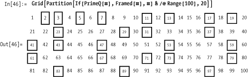
Once you become comfortable with functional programming, you will find all sorts of really nice applications of this general pattern. Here is a slick little demonstration borrowed from the Mathematica PrimeQ documentation for visually identifying the primes in the first 100 positive integers.

In the following, I apply the technique twice to create a presentation that shows the first 12 regular polygons, with the number of sides and the interior angles in degrees displayed in the center.

The first step is to generate a list of lists using Table. The innermost list (rows below) contains n equally spaced angles about a circle where n varies between 3 and 14. We can see this by inspecting angles in tabular form. Here, using Map is superior to Table if you want to use the computed table of angles in further steps in the computation. In my case, I just want to display them.

Since Polygon requires points, I compute them by mapping the Sin and Cos functions in parallel over each sublist by giving a level specification of {2} to Map. I show only the first three results below for sake of space.

The next pass uses the technique to create both the polygon and the inset with the number of sides and the interior angles. The use of Partition and GraphicsGrid is solely for formatting purposes.

See 2.5 Keeping Track of the Index of Each Item As You Map for a variation of Map called MapIndexed that gives you the position of an element as a second argument.

You want to apply a function over a list as with Map (/@), but the function requires the position of the item in the list in addition to its value.

Use MapIndexed instead of Map. Keep in mind that MapIndexed wraps the index in a list, so a common idiom is to use First[#2] to access the index directly. To show this, I first use an undefined function ff before showing a more useful application.

In[50]:= Clear[ff];
         MapIndexed[ff[#1, First[#2]] &, {a, b, c, d, e}]
Out[51]= {ff[a, 1], ff[b, 2], ff[c, 3], ff[d, 4], ff[e, 5]}

Imagine you want to raise the elements of a list to a power based on its position. You could not easily do this with Map, but MapIndex makes it trivial.

In[52]:= MapIndexed[#1^First[#2] &, {2,0,7,3}]
Out[52]= {2, 0, 343, 81}

This is not so contrived if you consider the problem of converting a list to a polynomial.

In[53]:= Plus @@ MapIndexed[#1x^First[#2] &, {2, 0, 7, 3}]
Out[53]= 2x + 7x3 + 3x4

Although MapIndexed is used less frequently than Map, it is a godsend when you need it, since it avoids the need to return to a procedural style when you want the position. I think you might agree the following procedural implementation is a bit uglier.

In[54]:=  Block[{poly = 0,
            list = {2, 0, 7, 3}},
           Do[
            poly = poly + list[[i]] x^i,
            {i, 1, Length[list]}
           ];
           poly]
Out[54]= 2 x + 7x3 + 3 x4

You may find it curious that MapIndexed wraps the position in a list, forcing you to use First to extract the index. There is a good reason for this convention: MapIndexed easily generalizes to nested lists such as matrices where the position has multiple parts. Here we use a variant of MapIndexed that takes a level specification as a third argument indicating the function ff should map over the items at level two. Here two integers are required to specify the position; thus, the list convention immediately makes sense.

In[55]:= MapIndexed[ff[#1, #2] &, {{a, b, c}, {d, e, f}, {g, h, i}}, {2}]
Out[55]= {{ff[a, {1, 1}], ff[b, {1, 2}], ff[c, {1, 3}]},
          {ff[d, {2, 1}], ff[e, {2, 2}], ff[f, {2, 3}]},
          {ff[g, {3, 1}], ff[h, {3, 2}], ff[i, {3, 3}]}}

As an application, consider a function for reading the positions of pieces on a chessboard. The board is a matrix with empty spaces designated by 0 and pieces designated by letters with subscripts B for black and W for white. We implement a function piecePos that can convert a piece and its position into a description that uses algebraic chess notation.

In[56]:=  Clear[piecePos]
          chessboard = {
              {0, 0, 0, 0, 0, 0, 0, 0},
              {0, 0, 0, 0, 0, 0, 0, 0},
              {0, 0, 0, 0, 0, 0, 0, 0},
              {0, 0, 0, 0, 0, 0, 0, 0},
              {NB, PW, NW, 0, 0, 0, 0, 0},
              {0, 0, 0, 0, 0, 0, 0, 0},
              {0, 0, QW, 0, 0, 0, 0, 0},
              {KB, 0, 0, 0, 0, 0, 0, 0}
             };

          toColor[B] = "Black";
          toColor[W] = "White";
          toPos[{x_, y_}] :=
           Module[{file = {"a", "b", "c", "d", "e", "f", "g", "h"}},
            file[[y]] <> ToString[x]]

          piecePos[Pc_, pos_] := {toColor[c], " Pawn ", toPos[pos]}
          piecePos[Nc_, pos_] := {toColor[c], " Knight ", toPos[pos]}
          piecePos[Bc_, pos_] := {toColor[c], " Bishop ", toPos[pos]}
          piecePos[Rc_, pos_] := {toColor[c], " Rook ", toPos[pos]}
          piecePos[Qc_, pos_] := {toColor[c], " Queen ", toPos[pos]}
          piecePos[Kc_, pos_] := {toColor[c], " King ", toPos[pos]}
          piecePos[0, _] := Sequence[]

MapIndexed will allow us to use piecePos to describe the whole board. Here, piecePos converts an empty space to any empty sequence, which Mathematica will automatically remove for us. Flatten is used to collapse unneeded nesting inherited from the chessboard’s representation as a list of lists.

In[68]:= Flatten[MapIndexed[piecePos, chessboard, {2}],1]
Out[68]= {{Black,  Knight, a5}, {White, Pawn, b5},
          {White,  Knight, c5}, {White, Queen, c7}, {Black, King, a8}}

You have a list and wish to apply some operation over a moving window of fixed size over that list.

Ignoring available special functions of Mathematica for a moment, you can attack this problem head-on by using Table in conjunction with a Part and Span (i.e., [[start;;end]]) to create the moving window (sublist) and Apply the desired function to each sublist. For example, use Mean if you want a moving average.

In[69]:=  array = RandomReal[{0, 10}, 20] ;

In[70]:=  Table[Mean @@ {array[[i ;; i + 4]]}, {i, 1, 16}]
Out[70]=  {3.13108, 3.27291, 4.31676, 5.41289, 5.98751, 5.6219, 5.8349, 5.52834,
           5.87892, 4.7862, 5.5245, 5.36589, 4.35811, 4.09389, 4.66446, 3.87226}

Here is a variation using Take.

In[71]:=  Table[Mean @@ {Take[array, {i, i + 4}]}, {i, 1,16}]
Out[71]=  {3.13108, 3.27291, 4.31676, 5.41289, 5.98751, 5.6219, 5.8349, 5.52834,
           5.87892, 4.7862, 5.5245, 5.36589, 4.35811, 4.09389, 4.66446, 3.87226}

A nonmathematical example uses the same technique to create successive pairs.

In[72]:=  Table[List @@ array[[i ;; i + 1]], {i, 1, 16}]
Out[72]=  {{5.14848, 4.21272}, {4.21272, 0.968604},
           {0.968604, 2.94497}, {2.94497, 2.38062}, {2.38062, 5.85762},
           {5.85762, 9.43197}, {9.43197, 6.44928}, {6.44928, 5.81804},
           {5.81804, 0.552592}, {0.552592, 6.92264},
           {6.92264, 7.89915}, {7.89915, 8.20219}, {8.20219, 0.354432},
           {0.354432, 4.24409}, {4.24409, 6.12958}, {6.12958, 2.86026}}

The solution illustrates the basic idea, but it is not very general because the function and window size are hard coded. You can generalize the solution like this:

In[73]:= moving[f_, expr_, n_] := Module[{len = Length[expr], windowEnd },
           windowEnd = Min[n, len] - 1;
           Table[Apply [f, {expr[[i;;i + windowEnd]]}], {i, 1, len - windowEnd}]]

Note that there is a built-in function, MovingAverage, that computes both simple and weighted moving averages. There is also a MovingMedian. You should use these instead of the solution given here if they are appropriate for what you need to compute.

Two special functions in Mathematica, ListConvolve and ListCorrelate, present the most general way to perform computations on sublists. These functions contain a myriad of variations, but it is well worth the added effort to familiarize yourself with them. I will present only ListConvolve because anything you can compute with one you can compute with the other, and the choice is just a matter of fit for the specific problem. Let’s ease in slowly by using ListConvolve to implement a moving average.

In[74]:= movingAvg[list_, n_] := ListConvolve[Table[1/n, {n}],list]

In[75]:= movingAvg[array, 5]
Out[75]= {3.13108, 3.27291, 4.31676, 5.41289, 5.98751, 5.6219, 5.8349, 5.52834,
          5.87892, 4.7862, 5.5245, 5.36589, 4.35811, 4.09389, 4.66446, 3.87226}

The first argument to ListConvolve is called the kernel. It is a list that defines a set of values that determines the length of the sublists and factors by which to multiply each element in the sublist. After the multiplication, each sublist is summed. This is shown more easily using symbols.

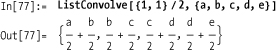
In[76]:= ListConvolve[{1, 1}, {a, b, c, d, e}]
Out[76]= {a + b, b + c, c + d, d + e}

Here I use a simple kernel {1,1}, which implies sublists will be size 2 and each element will simply be itself (because 1 is the identity). This yields a list of successive sums. In the moving average, the kernel was simply 1/n repeated n times since this results in the mean.

It’s easy to see how using an appropriate kernel gives a weighted moving average, but I won’t continue in this vein, because my goal is to demonstrate the generality of ListConvolve and, as I already said, MovingAverage does the trick.

The first bit of generality comes from Mathematica adding a third argument to ListConvolve that can be an integer k or a list {kL,kR}. Since using just k is equivalent to using {k,k}, I’ll only discuss the later case. It is best to start with some examples.

In[78]:= ListConvolve[{1, 1}, {a, b, c, d, e}, {1, 1}]
Out[78]= {a + e, a + b, b + c, c + d, d + e}

In[79]:= ListConvolve[{1, 1}, {a, b, c, d, e}, {1, -1}]
Out[79]= {a + e, a + b, b + c, c + d, d + e, a + e}

Hopefully you can guess the meaning of {kL,kR}; kL tells ListConvolve how much to overhang the kernel on the left of the list, and kR tells it how much to overhang the kernel on the right. Hence, it tells ListConvolve to treat the list as circular. The default value is {-1,1}, which means no overhang on either side.

Sometimes you do not want to treat the lists as circular, but rather as padded; hence, ListConvolve takes a fourth argument that specifies the padding.

In[80]:= ListConvolve[{1, 1}, {a, b, c, d, e}, {1, -1}, 1]
Out[80]= {1 + a, a + b, b + c, c + d, d + e, 1 + e}

I’ve rushed through these features a bit because the Mathematica documentation can fill you in on the details and because my real goal is to arrive at the version of ListConvolve that takes a fifth and sixth argument. This takes us back to the theme of this recipe, which is the idea of mapping arbitrary functions over moving sublists. Thus far, ListConvolve has been about mapping a very specific function, Plus, across a sublist defined by a kernel, which defines both the length of the sublist (matches length of kernel) and a set of weights to Times the individual elements (the elements of the kernel). The fifth argument allows you to replace Times with an arbitrary function, and the sixth argument allows you to replace Plus with an arbitrary function.

Here is the pair extraction function from the solution implemented using ListConvolve, shown here but using strings to emphasize that we don’t necessarily need to do math. I replace Times with the function #2&, which simply ignores the element from the kernel, and I replace Plus with List because that will form the pairs.

In[81]:= list = {"foo", "bar", "baz", "bing"};
         ListConvolve[{1, 1}, list, {-1, 1}, {}, #2&, List]
Out[82]= {{foo, bar}, {bar, baz}, {baz, bing}}

But sometimes you can make nice use of the kernel even in nonmathematical contexts. Here we hyphenate pairs using StringJoin with input kernel strings {"-",""} (consider that "" is the identity for string concatenation).

In[83]:= ListConvolve[{"-", ""}, list, {-1, 1}, {}, StringJoin, StringJoin]
Out[83]= {foo-bar, bar-baz, baz-bing}

Let’s consider another application. You have a list of points and want to compute the distances between successive pairs. This introduces a new wrinkle because the input list is two levels deep. ListConvolve assumes you want to do a two-dimensional convolution and will complain that the kernel does not have the same rank as the list. Luckily, you can tell ListConvolve to remain on the first level by specifying a final (seventh) argument.

In[84]:= points = RandomReal[{-1, 1}, {20,2}];
         ListConvolve[{1, 1}, points, {-1, 1}, {}, #2 &, EuclideanDistance, 1]
Out[85]= {1.49112, 0.764671, 0.789573, 0.941825, 0.933473, 1.05501,
          1.21181, 0.827185, 1.25728, 0.365742, 0.62815, 1.88344, 0.741821,
          1.13765, 0.719799, 0.643237, 1.60263, 0.93153, 1.33332}

Taking three points at a time, you can compute the area of successive triangles and draw them as well!

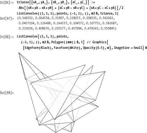
There is something a bit awkward about ListConvolve use cases where we essentially ignore the kernel. Readers familiar with the function Partition will immediately see a much shorter variation.

In[89]:= triarea @@@ Partition[points, 3, 1]
Out[89]= {0.549352, 0.064558, 0.31907, 0.228057, 0.308535, 0.561063,
          0.0457104, 0.126488, 0.164337, 0.104572, 0.107751, 0.581687,
          0.333659, 0.408676, 0.220177, 0.457996, 0.679265, 0.550845}

Partition and ListConvolve have many similar features, and with a bit of programming, you can implement ListConvolve in terms of Partition and vice versa. The one observation I can make in favor of ListConvolve is that it does the partitioning and function application in one fell swoop. This inspires the following compromise.

In[90]:= partitionApply[func_, list_, n_] :=
          ListConvolve[Array[1 &, n], list, {-1, 1}, {}, #2&, func, 1]

Above, Array is used to generate a kernel of the required size where 1& is the function that always returns 1.

In[91]:= partitionApply[triarea, points, 3]
Out[91]= {0.549352, 0.064558, 0.31907, 0.228057, 0.308535, 0.561063,
          0.0457104, 0.126488, 0.164337, 0.104572, 0.107751, 0.581687,
          0.333659, 0.408676, 0.220177, 0.457996, 0.679265, 0.550845}

But, lo and behold, the function we are looking for is actually buried inside the Developer' package! It’s called Developer'PartitionMap.

In[92]:= Developer'PartitionMap[triarea @@ # &, points, 3, 1]
Out[92]= {0.549352, 0.064558, 0.31907, 0.228057, 0.308535, 0.561063,
          0.0457104, 0.126488, 0.164337, 0.104572, 0.107751, 0.581687,
          0.333659, 0.408676, 0.220177, 0.457996, 0.679265, 0.550845}

I highly recommend reviewing the documentation for Partition, ListConvolve, and ListCorrelate in succession to get insight into their relationships. I spent a lot of time in my early Mathematica experience understanding how to use Partition but viewing ListConvolve and ListCorrelate as mysterious. If you find a need to use Partition in one of its advanced forms, you might be working on a problem where ListConvolve or ListCorrelate applies.

ListConvolve and ListCorrelate are frequently used in image-processing applications. See 8.5 Sharpening Images Using Laplacian Transforms. Also see 2.12 Building a Function Through Iteration, in which I use ListConvolve for a traveling salesperson problem.

A complicated piece of functional code can become deeply nested and, as a result, hard to read. You want to collapse some of these levels of nesting without introducing intermediate variables. Of course, readability is in the eye of the beholder, so a closely related problem is making sure you can understand this style when you see it in the wild.

Many Mathematica veterans prefer a functional style of programming that makes liberal use of prefix notation, which uses the @ symbol to compose functions, and postfix notation, which uses //. Let’s consider a simple program that looks for primes of the form 2 ⁿ ± 1 up to some limiting value of nmax.

In[93]:= somePrimes[nmax_] :=
           Select [Union [Flatten [Table [{2^n - 1, 2^n + 1}, {n, 0, nmax}]]], PrimeQ];
         somePrimes[
          5]
Out[94]= {2, 3, 5, 7, 17, 31}

As a first step, you can eliminate some levels of nesting by using @.

In[95]:= somePrimes[nmax_] :=
          Select[Union@Flatten@Table[{2^n - 1, 2^n + 1}, {n, 0, nmax}], PrimeQ]
         somePrimes[5]
Out[96]= {2, 3, 5, 7, 17, 31}

You can further emphasize that this program is about finding primes by using functional composition with Select. This brings the PrimeQ test to the front.

In[97]:= somePrimes[nmax_] := Select[#, PrimeQ] & @
           Union@Flatten@Table[{2^n - 1, 2^n + 1}, {n, 0, nmax}]
         somePrimes[
          5]
Out[98]= {2, 3, 5, 7, 17, 31}

The use of postfix is perfectly valid on the left-hand side, although you are less likely to see this style widely used.

In[99]:= somePrimes@nmax_:=
          Select[#, PrimeQ] & @ Union@Flatten@Table[{2^n - 1, 2^n + 1}, {n, 0, nmax}]

A functional purist might go further and make somePrimes a pure function, but most would agree this goes way too far in this instance! Still, you should know how to read code like this, because you will come across it, and there are cases where it makes sense.

In[100]:= Clear[somePrimes];
          somePrimes = (Select[#, PrimeQ] & @
                Union@Flatten@Table[{2^n - 1, 2^n + 1}, {n, 0, #}]) &;
          somePrimes[
           5]
Out[102]= {2, 3, 5, 7, 17, 31}

The uninitiated could make an argument that the first form of somePrimes was more understandable to them than any of the later ones. First, let me say that there is no reward in heaven for coding in a specific style, so don’t feel the need to conform to a particular fashion. Your programs won’t run faster just because you use a terser syntax. Having said that, I now defend the merits of this particular style. Let me repeat the version that I think strikes the right balance.

In[103]:= Clear[somePrimes];
          somePrimes[nmax_] :=
           Select[#, PrimeQ] & @ Union@Flatten@Table[{2^n - 1, 2^n + 1}, {n, 0, nmax}]

First, use of symbols like @ should not be a real barrier. After all, such symbolic forms of expression are pervasive. Every first grader knows what 1 + 1 or $15 means. Symbolic operators are not inherently mysterious after you are exposed to them.

However, the primary goal and claim is readability. This expression can be read as "select the primes of the union of the flattening of the table of pairs {2^n-1, 2^n+1} with n ranging from 0 to nmax". As I stated in the solution, the most relevant aspect of this program is that it selects primes. Having a language that gives you the freedom to express programs in a way that emphasizes their function is really quite liberating in my opinion.

The flip side of emphasis by pushing functions forward is deemphasis by pushing ancillary detail toward the end. This is one of the roles of postfix //. Common uses include formatting and timing. Here the main idea is taking the last value of somePrimes[500]. The fact that you are interested in the timing is likely an afterthought, and you may delete that at some point. Placing it at the end makes it easy to remove.

In[105]:= Last@somePrimes[500] // Timing
Out[105]= {0.113328, 170141183 460469 231731687 303 715 884105 727}

Likewise, formatting is a convention that does not change meaning, so most users tag formatting directives at the end.

  In[106]:=  10.00 + 12.77 - 36.00 - 42.01 // AccountingForm
Out[106]//AccountingForm=
              (55.24)

Note that @ has high precedence and associates to the right, whereas // has low precedence and associates to the left. The precedence is suggested by the way the frontend typesets expressions with @ containing no space to suggest tight binding, while // expressions are spaced out to suggest loose binding and lower precedence.

In[107]:= a@b@c//f@d//e
Out[107]= e[f[d][a[b[c]]]]

It’s worth mentioning that Postfix and Prefix will convert standard functional form to the shortened versions.

In[108]:= Prefix[f[1]]
Out[108]= f@1

In[109]:= Postfix[f[1]]
Out[109]= 1//f

Additional perspectives on this notation can be found in the essay The Concepts and Confusions of Prefix, Infix, Postfix and Fully Nested Notations by Xah Lee at http://bit.ly/t6GoC.

Readers interested in functional programming styles should google the term Pointfree to learn how the ideas discussed here manifest themselves in other languages, such as Haskell.

You want to define a family of functions differentiated by an index or indices.

Use indexed heads or subscripts.

In[110]:=  ClearAll[f];
           f[1][x_, y_] := 0.5 * (x + y)
           f[2][x_, y_] := 0.5 * (x - y)
           f[3][x_, y_] := 0.5 * (y - x)
In[114]:=  Table[f[Randomlnteger[{1, 3}]][3, 2], {6}]
Out[114]=  {2.5, -0.5, -0.5, -0.5, 2.5, 0.5}

The mathematician in you might prefer using subscripts instead.

In[115]:=  ClearAll[f];
           f1[x_, y_] := 0.5 * (x + y)
           f2[x_, y_] := 0.5 * (x - y)
           f3[x_, y_] := 0.5 * (y - x)
In[119]:=  fRandomInteger[{1,3}][3, 2]
Out[119]=  0.5

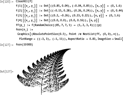
In Stan Wagon’s Mathematica in Action (W.H. Freeman), there is a study of iterated function systems that are nicely expressed in terms of indexed functions. This is a variation of his code that takes advantage of the new RandomChoice function in Mathematica 6. The fernlike structure emerges out of a nonuniform distribution of function selections.

You are not restricted to indexing functions by integers. Here are some variations that are possible.

In[128]:= g[1, 1][x_, y_] := x + 2 y
          g[weird][x_, y_] := Exp[Sin[x] Tan[y]]
          g[1 + 2I] := x + 2 y I

You want to understand and create programs that use Fold[] as an alternative to explicit recursion.

Consider the following simple recursive definition for a summation function.

In[131]:= mySum[{}] := 0
          mySum[1_] := First[1] + mySum[Rest[1]]

In[133]:= mySum[{1, 2, 3, 4, 5}]
Out[133]= 15

This function can easily be translated to a nonrecursive implementation that uses Fold[].

In[134]:= mySum2[1_] := Fold[#1 + #2 &, 0, 1]

In[135]:= mySum2[{1, 2, 3, 4, 5}]
Out[135]= 15

The function Fold[f, x, {a1,a2,...,aN}] computes f[f[f[x,a1],a2],...,aN]. It is a simple enough definition to understand, but it is not always clear to the uninitiated when such a function might be useful. It turns out that there is a relationship between Fold and certain common kinds of recursive functions. Consider the following abstract recursive structure.

g[{}] = x
g[1_] = f[First[1], g[Rest[1]]]

When a function g has this recursive structure in terms of another function f, then it can easily be translated into a nonrecursive function using Fold, provided f is associative. If f is not associative, then you may need to reverse the list l before passing to Fold.

g[1_] = Fold[f[#1,#2]&,x,l]

Here is an example that shows that the functionality of Map can be implemented in terms of Fold. First start with your own recursive definition of Map.

In[136]:= myMap[_, {}] := {}
          myMap[f_, l_] := Prepend[myMap[f, Rest[1]], f[First[1]]]

The translation requires reversing the list because prepending the application of f to a list is clearly not associative.

In[138]:= myMap2[f_, l_] := Fold[Prepend[#1, f[#2]] &, {}, Reverse[1]]

Here is a test of the recursive implementation, first on an empty list, then on a nonempty one.

Now the Fold version.

Before considering more useful applications of Fold, I need to clear up some potential confusion with folding implementations from other languages. In Haskell, there are functions called foldl and foldr, which stand for fold left and fold right, respectively. Mathematica’s Fold is like foldl.

In[143]:= (*This is like Haskell's foldr.*)
          foldr[f_, v_, {}] := v
          foldr[f_, v_, l_] := f[First[1], foldr[f, v, Rest[1]]]

In[145]:= (*This is like Haskell's foldl and Mathematica's Fold.*)
          foldl[f_, v_, {}] := v
          foldl[f_, v_, l_] := foldl[f, f[v, First[1]], Rest[1]]

These various folds will give the same answer if the function passed is associative and commutative.

In[147]:= foldr[Plus, 0, {1,2,3}]
Out[147]= 6

In[148]:= foldl[Plus, 0, {1,2,3}]
Out[148]= 6

In[149]:= Fold[Plus, 0, {1, 2, 3}]
Out[149]= 6

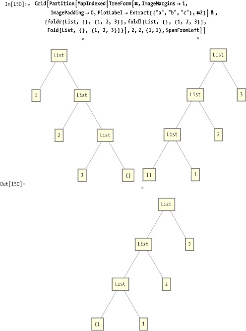
To visualize the difference between foldr and foldl, consider the trees produced by using the List function. Trees labeled b and c are the same, confirming the equivalence of Haskell’s foldl and Mathematica’s Fold.

You can use the relationship between Fold and recursion to analyze more complicated use cases. For example, the Mathematica documentation provides an example of using Fold to find all the unique sums of a list of numbers.

In[151]:= Fold[Union[#1, #1 + #2] &, {0}, {1, 2, 7}]
Out[151]= {0, 1, 2, 3, 7, 8, 9, 10}

When I first saw this, it was not immediately obvious to me why the solution worked. However, by converting to the recursively equivalent solution, it is easier to analyze what is happening.

In[152]:=  uniqueSums[{}] :=  {0}
           uniqueSums[1_] :=
            Union[{First[1]}, uniqueSums[Rest[1]], First[1] + uniqueSums[Rest[1]]]
In[154]:=  uniqueSums[{1, 2, 7}]
Out[154]=  {0, 1, 2, 3, 7, 8, 9, 10}

The first rule is obvious. The sum of the empty list is zero. The second rule says that the unique sums of a list are found by taking the union of the first element of the list, the unique sums of the rest of the list, and the sum of the first element and the unique sums of the rest of the list. The last part of the union (First[1] + uniqueSums [Rest[1]]) provided me with the key insight into why this example worked. It is a sum of a scalar and a vector and provides the sum of the first element with all other combinations of sums of the remaining elements. It is obvious that the recursive translation, as written, is suboptimal because the recursive call is made twice (this could easily be fixed with a local variable), but the point here was to use the recursive function as a tool to analyze the meaning of the Fold implementation.

FoldList is a variant of Fold that returns all intermediate steps of the Fold in a list. Refer to the Mathematica documentation for details.

Nest and NestList also repeatedly apply a function to an expression, but the repetitions are controlled by an integer n. See 2.11 Computing Through Repeated Function Application.

NestWhile and NestWhileList apply a function as long as a test condition remains true. See 2.11 Computing Through Repeated Function Application.

You need to build up a list piece by piece during an iterative or recursive computation.

An obvious solution to this problem is to use the function AppendTo[s, elem]; however, AppendTo should be avoided for performance reasons. Instead, use Reap and Sow. Here is a simple factorial function that collects intermediate results using Reap and Sow.

In[155]:= factorialList[n_Integer/; n ≥ 0] := Reap[factorialListSow[n]]
          factorialListSow[0] := Sow[1]
          factorialListSow[n_]:= Module[{fact}, Sow[n * factorialListSow[n - 1]]]

In[158]:= factorialList[8]
Out[158]= {40320, {{1, 1, 2, 6, 24, 120, 720, 5040, 40320}}}

Reap and Sow cause confusion for some, possibly because there are few languages that have such a feature built in. Simply think of Reap as establishing a private queue and each Sow as pushing an expression to the end of that queue. When control exits Reap, the items are extracted from the queue and returned along with the value computed by the code inside the Reap. I don’t claim that Reap and Sow are implemented in this way (they might or might not be), but thinking in these terms will make you more comfortable with their use.

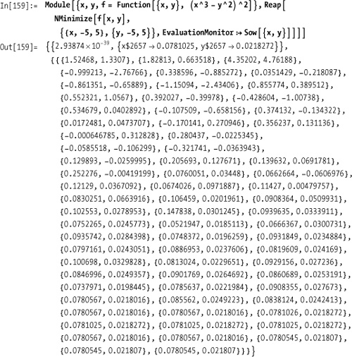
Reap and Sow are often used as evaluation-monitoring functions for numerical algorithms. FindRoot, NDSolve, NIntegrate, NMinimize and NSum allow an optional EvaluationMonitor or StepMonitor where Reap and Sow can come in handy.

Reap and Sow also can be used to build up several lists by specifying tags with Sow and patterns that match those tags in Reap. Here you create a three-way partitioning function using an ordering function by sowing values with tags -1, 0, or 1, depending on the relation.

In[160]:=  partition[1_, v_, comp_ ] := Flatten /@ Reap[
               Scan[
                Which[comp[#, v], Sow[#, -1],
                  comp[v, #], Sow[#, 1], True, Sow[#, 0]] &, l],
               {-1, 0, 1}][[2]]
In[161]:=  partition[{3, 5, 7, 9, 2, 4, 6, 8, 3, 4}, 4, Less]
Out[161]=  {{3, 2, 3}, {4, 4}, {5, 7, 9, 6, 8}}

Our queue analogy easily extends to this case by assuming Reap establishes a separate queue for each pattern and Sow chooses the matching queue.

Reap and Sow are used in the tree traversal algorithms in 3.11 Implementing Trees and Traversals Using Lists.

You want to understand the types of computations you can perform using the Nest family of functions (Nest, NestList, NestWhile, NestWhileList).

Many problems require repeated application of a function for a specified number of times. One example that is familiar to most people is compounded interest.

In[162]:= compoundedInterest[principal_, rate_, years_, n_] :=
           Nest[# (1.0 + rate/n) &, principal, years n]

As expected, the principal grows in value quicker the more times the interest is compounded per year.

In[163]:= Table[compoundedInterest[1000, 0.05, 10, n], {n, {1, 2, 4, 12, 365}}]
Out[163]= {1628.89, 1638.62, 1643.62, 1647.01, 1648.66}

Another classic application is fractals. Here I use Nest to generate one side of the Koch snowflake. The rule for creating the snowflake is to take the line segment, divide it into three equal segments, rotate copies of the middle segment Pi/3 and -Pi/3 radians from their ends to form an equilateral triangle, and then remove the middle section of the original line segment. This is implemented literally (but not efficiently) by iterating a replacement rule using Nest. We cover these rules in Chapter 4.

If you are interested in the intermediate values of the iteration, NestList is the answer. Suppose you want to see all rotations of a shape through d radians. Here I use NestList to rotate clockwise and translate a square with a dot in its corner through angle d until at least 2Pi radians (360 degrees) are covered.

NestWhile and NestWhileList generalize Nest and NestList, respectively, by adding a test predicate to determine if the iterative application of the function should continue. In addition to the test, an upper limit can be specified to guarantee the iteration terminates in a given number of steps if the test does not terminate it first. Here is an application that searches for a tour in a traveling salesperson problem (TSP) that is less than some specified distance. The cities are numbered 1 through n, and the distances are represented as a sparse matrix.

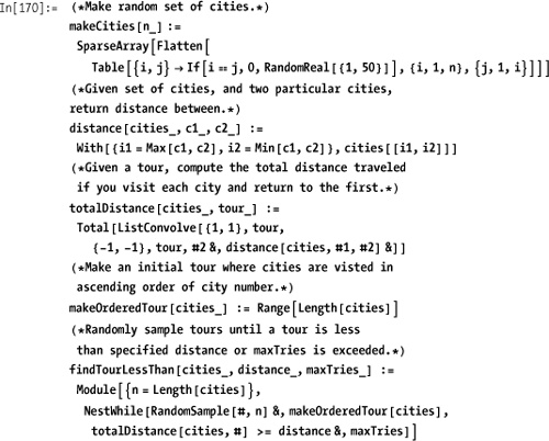
The algorithm is not very intelligent, but it nicely demonstrates NestWhile. First I make a random set of 10 cities and see the distance of the ordered tour.

In[175]:= cities = makeCities[10];
          dist = totalDistance[cities, makeOrderedTour[cities]]
Out[176]= 273.898

Now I see if I can find a better tour that is better than 80% of the ordered tour in 100,000 tries.

In[177]:= findTourLessThan[cities, 0.80dist, 100000]
Out[177]= {9, 5, 10, 2, 6, 8, 3, 7, 1, 4}

You can see that it was successful!

In[178]:= totalDistance[cities, %]
Out[178]= 300.754

The replacement rules used in the Koch snowflake are covered in Chapter 4.

In 12.16 Creating Stochastic Simulations, NestList is used to drive a simulation.

The TSP example used ListConvolve to compute the distance of a tour. See 2.6 Mapping a Function over a Moving Sublist.

You want to construct a higher-order function from explicit iteration of a lower-order function.

This is a good application for Nest. For example, you can pre-expand terms in Newton’s method for .

In[179]:=  Clear[f, x, y, z, n, terms];
           makeSqrtNewtonExpansion[n_, terms_Integer: 4] :=
            Function[x,
             Evaluate[Together[Nest[Function[z, (z + n / z) / 2],x, terms]]]]

In[181]:=  sqrt2 = makeSqrtNewtonExpansion[2, 4]
Out[181]=  Function[x$, (256 + 15 360 x$2 + 116480 x$4 +
               256 256 x$6 + 205 920 x$8 + 64 064 x$10 + 7280 x$12 + 240 x$14 + x$16)/
             (16 x$ (2 + x$2) (4 + 12 x$2 + x$4) (16 + 224 x$2 + 280 x$4 + 56 x$6 + x$8))]

We are left with a function that will converge quickly to sqrt[2] when given an initial guess. Here we see it takes just four iterations to converge.

In[182]:= FixedPointList[sqrt2, 1`40]
Out[182]= {1.000000000000000000000000000000000000000,
           1.41421356237468991062629557889013491012,
           1.4142135623730950488016887242096980786,
           1.414213562373095048801688724209698079}

Code generation is a powerful technique; the solution shows how Function and Nest can be used with Evaluate to create such a generator. The key here is the use of Evaluate, which forces the Nest to execute immediately to create the body of the function. Later, when you use the function, you execute just the generated code (i.e., the cost of the Nest is paid only during generation, not application).

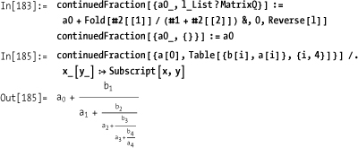
Fold can also be used as a generator. Here is an example of constructing a continued fraction using Fold adapted from Eric W. Weisstein’s "Continued Fraction" from MathWorld ( http://bit.ly/35rxJF ).

You want to compose one or more functions to produce a new function, with the added ability to easily invert the new function.

Use Composition to build a new function f1[f2[f3...[x]]] from f1, f2, f3... and InverseFunction to convert the composition to ...f3–1[f2–1[f1–1[x]]].

In[186]:= f = Composition[Exp, Cos]
Out[186]= Composition[Exp, Cos]

In[187]:= result = f[0.5]
Out[187]= 2.40508

In[188]:= Exp[Cos[0.5]]
Out[188]= 2.40508

If the composed functions are invertible, you can compute the inverse of the composition.

In[189]:= InverseFunction[f][result]
Out[189]= 0.5

The Mathematica 6 documentation for Composition is not very compelling. It lists the following examples of usage:

  In[190]:=  (*Create a sum of numbers to be displayed in held form.*)
             Composition [HoldForm, Plus] @@ Range[20]
             1 + 2 + 3 + 4 + 5 + 6 + 7 + 8 + 9 + 10 + 11 + 12 + 13 + 14 + 15 + 16 + 17 + 18 + 19 + 20
  Out[190]=  1 + 2 + 3 + 4 + 5 + 6 + 7 + 8 + 9 + 10 + 11 + 12 + 13 + 14 + 15 + 16 + 17 + 18 + 19 + 20
  
  In[192]:=  (*Tabulate square roots of values without using auxiliary variables.*)
             TableForm[Composition[Through, {Identity, Sqrt}] /@ {0, 1.0, 2.0, 3.0, 4.0}]
Out[192]//TableForm=
             0   0
             1.  1.
             2.  1.41421
             3.  1.73205
             4.  2.

Although these are certainly examples of usage, they are not compelling because the same results can be achieved without Composition and, to my tastes, more simply.

In[193]:= HoldForm[Plus[##]] & @@ Range[20]
Out[193]= 1 + 2 + 3 + 4 + 5 + 6 + 7 + 8 + 9 + 10 + 11 + 12 + 13 + 14 + 15 + 16 + 17 + 18 + 19 + 20

This is an example of 2.4 Mapping Multiple Functions in a Single Pass.

   In[194]:= {Identity[#], Sqrt[#]} & /@ {0, 1.0, 2.0, 3.0, 4.0} // TableForm
Out[194]//TableForm=
             0   0
             1.  1.
             2.  1.41421
             3.  1.73205
             4.  2.

For some time I thought that Composition was just a curiosity that might appeal to some mathematically minded folks on aesthetic grounds but otherwise did not add much value. This was before I understood how Composition can work together with InverseFunction. When you have an arbitrary composition of functions, InverseFunction will produce an inverse of the composition by inverting each component and reversing the order of application. In the case of the example in the preceding Solution section, you get the following:

In[195]:= InverseFunction[Composition[Exp, Cos]]
Out[195]= Composition[ArcCos, Log]

Unfortunately, mathematical functions often are not invertible, so this particular example will not always work given an arbitrary list of functions. But the really cool thing is that the functions need not be mathematical or perfectly invertible as long as you tell Mathematica you know what you’re doing by defining the inverses of your custom functions!

You can see that Mathematica has no idea what the inverse of RotateRight is, even though it is obvious that for a list it is RotateLeft.

In[196]:=  InverseFunction[RotateRight][{1, 2, 3}]
Out[196]=  RotateRight(–1) [{1, 2, 3}]

But you can define your own version and its inverse by using upvalues (see DownValues and UpValues).

In[197]:= ClearAll[reverse, rotateRight];
          rotateRight[list_List] := RotateRight[list]
          (*Define an UpValue for inverse of rotateRight.*)
          InverseFunction[rotateRight] ^:= RotateLeft[#1] &
          reverse[list_List] := Reverse[list]
          (*Clearly, reverse is its own inverse.*)
          InverseFunction[reverse] ^:= reverse[#] &

Now, given an arbitrary composition of these functions, we are guaranteed the ability to produce its inverse with no effort at all! I find that compelling, don’t you?

In[202]:= tr1 = Composition[reverse, rotateRight, rotateRight];

In[203]:= v = tr1[{1, 2, 3, 4, 5, 6}]
Out[203]= {4, 3, 2, 1, 6, 5}

In[204]:= InverseFunction[tr1][v]
Out[204]= {1, 2, 3, 4, 5, 6}

The obvious implication of this simple example is that if you define a set of functions and inverses, then given an arbitrary composition of those functions, you will always have the undo operation handy. Further, you get partial undo via Drop.

In[205]:= (*Drop one level of undo.*)
          Drop[InverseFunction[tr1], 1][v]
Out[205]= {6, 1, 2, 3, 4, 5}

In 2.7 Using Prefix and Postfix Notation to Produce More Readable Code we discussed composing functions using prefix operator @. The following illustrates the relationship:

In[206]:= Composition[f1, f2, f3][x] === f1@f2@f3@x
Out[206]= True

ComposeList returns the list of results computed by successive compositions of a given list of functions. See the Mathematica documentation.

You want to create expressions with persistent private state, behavior, and identity, but Mathematica does not directly support Lisp-like closures or object-oriented programming.

Note

The techniques described in this section fall a bit outside garden-variety Mathematica; some purists may frown on using techniques that make Mathematica feel like a different language. They might argue that Mathematica has enough features to solve problems and that users are better off mastering these rather than trying to morph the language into something else. I think this advice is generally sound. However, Mathematica is a system for multiparadigm programming as well as a system for research and exploration. So if you are interested, as I am, in exploring software development concepts for their own sake, I think you will find this recipe useful in stimulating new ideas about what Mathematica can do.

Create a symbol called closure with attributes HoldAll and with the form closure [var_List, val_List, func_List]. Create an evaluation function for closures that executes in a private environment provided by Block and returns the result and a new closure that captures any state changes that occurred during the evaluation.

In[207]:= SetAttributes[closure, HoldAll];
          SetAttributes [evaluate, HoldFirst];
          evaluate[f_,  closure[vars_, vals_, funcs_]] := Block[vars, vars = vals;
            Block[funcs, {f, closure[vars, Evaluate[vars], funcs]}]]

You can now use this machinery to create a counter.

In[210]:= ClearAll[makeCounter, counter];
           makeCounter[init_] :=  With[{v = init}, closure[{x}, {v},
              {incr = Function[x = x + 1], decr = Function[x = x - 1],
               reset = Function[v, x = v], read = Function[x]}]]
           counter = makeCounter[0]
Out[212]= closure[{x}, {0}, {incr = (x = x + 1) &,
            decr = (x = x - 1) &, reset = Function [v, x = v], read = x&}]

From a syntactic point of view, the implementation is only half done, but it is usable (see the following Discussion for the icing on the cake).

In[213]:= {val, counter} = evaluate[incr[], counter]; val
Out[213]= 1

When you evaluate again, you see that the state change persisted.

In[214]:= {val, counter} = evaluate[incr[], counter]; val
Out[214]= 2

Notice that even though the closure contains a free variable x, changes to x in the global environment do not impact the closure.

In[215]:= x = 0;
          {val, counter} = evaluate[incr[], counter]; val
Out[216]= 3

However, you can reset the counter through the provided interface. You can also decrement it and read its current value.

In[217]:= {val, counter} = evaluate[decr[], counter]; val
Out[217]= 2

In[218]:= {val, counter} = evaluate[reset[7], counter]; val
Out[218]= 7

In[219]:= {val, counter} = evaluate[read[7], counter]; val
Out[219]= 7

In computer science, a closure is a function that closes over the lexical environment in which it was defined. In some languages (e.g., Lisp, JavaScript), a closure may occur when a function is defined within another function, and the inner function refers to local variables of the outer function. Mathematica cannot do this in a safe way (as discussed here), hence the solution.

The solution presented is a bit awkward to use and read and, thus, would be easy to dismiss as a mere curiosity. However, we can use an advanced feature of Mathematica to make the solution far more compelling, especially to those readers who come from an object-oriented mind-set. One problem with the solution is that you need to deal with both the returned value and the returned closure. This is easy to fix by defining a function call that hides this housekeeping.

In[220]:= SetAttributes[call, HoldAll];
          call[f_, c_] :=  Module[{val}, {val, c} = evaluate[f, c]; val]

This simplifies things considerably.

In[222]:= val = call[decr[], counter]
Out[222]= 6

But we can go further by adding some syntactic sugar using the Notation facility.

Now you can write code like this:

You can use an existing closure to create new independent closures by creating a clone method. This is known as the prototype pattern.

In[228]:= clone[closure[vars_, vals_, funcs_]] :=
           clone[closure[vars, vals, funcs], vals]
          clone[closure[vars_, vals_, funcs_], newVals_] :=
           With[{v = newVals}, closure[vars, v, funcs]]

In[230]:= counter2 = clone[counter] (*Clone existing state.*)
Out[230]= closure[{x}, {1}, {incr = (x = x + 1)&,
            decr = (x = x - 1) &, reset = Function[v, x = v], read = x &}]

In[231]:= counter3 = clone[counter, {0}]
           (*Clone structure but initialize to new state.*)
Out[231]= closure[{x}, {0}, {incr = (x = x + 1)&,
            decr = (x = x - 1) &, reset = Function [v, x = v], read = x &}]

You can see these counters are independent from the original counters (but they do share the same functions, so they don’t incur much additional memory overhead).

It is instructive to compare this solution with other languages that support closures. In JavaScript, a closure over an accumulator can be created like this:

javascript
             function counter (n) {
                 return function (i) {return n += i}
                 }

Let’s see what happens if we attempt the same approach in Mathematica.

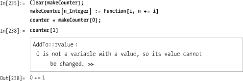
This was doomed from the start because n is not a free variable that can be closed over by Function. But let’s try something else.

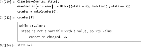
This fails because state is only defined while the block is active, because Block is a dynamic scoping construct and closures require lexical scoping. You might recall that Module is a lexical scoping construct; perhaps we would have better luck with that.

In[243]:=  Clear[makeCounter, state];
           makeCounter[n_Integer] := Module[{state = n}, Function[i, state += i]]
           counter = makeCounter[0];

In[246]:=  counter[1]
Out[246]=  1

In[247]:=  counter[1]
Out[247]=  2

This seems to work, but it has a flaw that you can see if you inspect the value of counter.

In[248]:= counter
Out[248]= Function[i$, state$2811 += i$]

The variable we called state has now morphed into something called state$< some number >. The point here is that Module implements lexical scope by synthesizing a global variable that is guaranteed not to be defined already, but that variable is not protected in any way and could be changed by the user. This is not esthetically pleasing and is not at all what is happening in the JavaScript or Lisp equivalents.

The solution in this recipe uses a different tactic. It uses the HoldAll attribute to create a container for the lexical environment of the closure. Because the variables and functions are held in unevaluated form, it makes no difference if there are global symbols with the same names. When it comes time to evaluate the closure, the evaluate function builds up a Block on the fly to create local instances of the variables and another Block to create local instances of the functions. It then binds the stored values of the variables and functions to these locals and calls the appropriate locally defined function.

What practical value are closures within the context of Mathematica? Clearly, creating a counter is too trivial. However, even the simple counter example shows some promising features of this technique. First, had we implemented the counter as a simple global variable, it could be used accidentally for some purpose inconsistent with the behavior of a counter. By encapsulating the counter in the closure, we restrict access to its state and the interface exposed by the closure becomes the only way to manipulate it. Further, the interface can be easily inspected because it is carried around inside the closure.

Mathematica 6’s Dynamic feature provides the context for a compelling application of closures. Let’s say you want to create a graphic that can be dynamically updated under programmatic control (rather than user control, for which you would use Manipulate instead). One way to do this is to define variables for all the aspects of the graphic that you need to change and wrap the graphic in a Dynamic function.

You then write Mathematica code that manipulates the variables as necessary to dynamically update the drawing. This is all well and good for a simple example with two shapes and four degrees of freedom, but imagine if you were doing this as part of a simulation that had hundreds of shapes with hundreds of degrees of freedom. Clearly, you would want a way to encapsulate all those variables behind an interface that made sense for the simulation. This closure facility can do just that.

In[251]:= ClearAll[shapeCtrl]
          shapeCtrl = closure[{rectX, rectY, rectAngle, circR}, {1, 2, 10 Degree, 1},
            {rotate = Function[a, rectAngle += a],
             grow = Function[r, rectX *= r; rectY *= r],
             rectCorner = Function[{rectX, rectY}],
             angle = Function[rectAngle],
             radius = Function[circR]}]
Out[252]= closure [{rectX, rectY, rectAngle, circR},
           {1, 2, 10 °, 1}, {rotate = Function[a, rectAngle += a],
            grow = Function [r, rectX *= r; rectY *= r],
            rectCorner = {rectX, rectY} &, angle = rectAngle &, radius = circR &}]

In[253]:= closure[{rectX, rectY, rectAngle, circR},
           {1, 2, 10 °, 1}, {rotate = Function [a, rectAngle += a],
            grow = Function [r, rectX *= r; rectY *= r],
            rectCorner = {rectX, rectY}&, angle = rectAngle&, radius = circR&}]
Out[253]= closure [{rectX, rectY, rectAngle, circR},
           {1, 2, 10 °, 1}, {rotate = Function [a, rectAngle += a],
            grow = Function [r, rectX *= r; rectY *= r],
            rectCorner = {rectX, rectY}&, angle = rectAngle&, radius = circR&}]

Here you define a closure, called shapeCtrl, over the same graphic but expose only two functions, rotate and grow, that are capable of changing the state. The other functions are strictly for returning the values for use in the graphic. You now specify the dynamic graphic in terms of the shape controller closure.

By its nature, dynamic content does not lend itself to static print demonstration, but we compensate by showing the result of each transform in the figure.

Figure 2-1. Transformations snapshots of the graphics

It could be argued that this recipe has crossed the boundary of the traditional definition of a closure and moved toward the capabilities of object-oriented programming. This is no accident, since there is a relationship between closures and objects, in that closures can be used to implement object-oriented programming, and languages like C++ can implement closures in terms of objects with operator(). However, a full-blown, object-oriented implementation would have to provide additional features not implemented by this recipe. Inheritance is the most obvious, but there are others (e.g., different access levels for functions and data). I prefer to think of this implementation as souped-up closures rather than dumbed-down objects, but you can think of them in whichever way makes the most sense to you. My feeling is that more traditional closures that act like single functions don’t provide enough bang for the buck. In any case, the simpler, traditional form can be implemented in terms of the richer form demonstrated in this recipe. Here is one way to do it.

In[255]:= (*First define a closure with a
           single function and assign to a variable.*)
          incr = closure[{x}, {0}, {incr = Function[x = x + 1]}]
Out[255]= closure[{x}, {0}, {incr = (x = x + 1) &}]

In[256]:= (*Then define a function pattern in terms of the same closure
           but with a Blank where the state variables would reside.*)
          closure[{x}, {_}, {incr = Function[x = x + 1]}] [] := call[incr[], incr]

In[257]:= (*Now, whenever the variable is used like a function,
          it will invoke the call on the closure.*)
          incr[]
Out[257]= 1

In[258]:= incr[]
Out[258]= 2

In[259]:= incr[]
Out[259]= 3

The Wikipedia entry for closures ( http://bit.ly/T9vhN ) is a good place to start learning more about this concept because it contains links to some useful papers and implementations in other languages.

You want to emulate the ability of other functional languages to automatically convert functions of multiple arguments into higher-order functions with a single argument.

Note

This recipe is more of theoretical interest to functional programming aficionados than of practical use for everyday Mathematica development. The techniques employed are of more general interest, but you may need to consult Chapter 4 if you are unfamiliar with patterns and replacement rules.

Mathematica does not support implicit currying like Haskell does, but you can use this solution to create functions that curry implicitly. Refer to the next section, Solution, if you are unfamiliar with currying.

Currying is the process of transforming a function that takes multiple arguments into a function that takes just a single argument and returns another function if any arguments are still needed. In languages that implicitly curry, you can write code as follows:

In[267]:= f1 = f[10]
Out[267]= f[10]

In[268]:= f2 = f1[20]
Out[268]= f[10][20]

In[269]:= f2[30]
Out[269]= f[10][20][30]

This is legal in Mathematica, but notice that when all three arguments are supplied, the function remains in unevaluated curried form. This is not the effect that you typically want. It is possible to manually uncurry by using ReplaceAllRepeated (//.) to transform the curried form to normal form.

The function Curry in the solution works as follows. It builds up an expression that says, "See if the specified function (first argument) with the specified parameters (second argument) will evaluate (ValueQ); if so, evaluate it. Otherwise, return the curried version of the function within a lambda expression using the Curry function itself." To add to the trickery, this expression needs to be built up in the context of a Hold to keep everything unevaluated until it can be transformed into a format where the ValueQ test and evaluation are in uncurried form. However, the lambda function part must remain in curried form, so we use z as a placeholder for a second round ReplaceAll (/.) that injects the curried form, instead of z.

I’ll be the first to admit this is tricky, but if you are tenacious (and perhaps look ahead to some of the recipes in Chapter 4), you will be rewarded with a deeper understanding of how powerful Mathematica can be at bootstrapping new behaviors. One way to get a handle on what is happening is to execute a version of Curry that does not release the Hold. This allows you to inspect the result at each stage before it is evaluated.

When the Hold is released, ValueQ[f[10]] will return false, so we will return a Function (&) that curries f[10] with yet to be supplied arguments ##1.

In[272]:= CurryHold[f, 10]
Out[272]= Hold[If[ValueQ[f[10]], f[10], Curry[f[10], ##1] &]]

When this Hold is released, ValueQ will also fail because there is no two-argument version of f, and we get a further currying function on f[10][20] that is ready for more arguments ##1.

In[273]:= CurryHold[f1, 20]
Out[273]=  Hold[If[ValueQ[f[10, 20]], f[10, 20], Curry [f[10][20], ##1] &]]

Finally, by supplying a third argument, we get an uncurried function f[10,20,30] that will evaluate; so ValueQ succeeds, and the uncurried version is evaluated.

In[274]:= CurryHold[f2, 30]
Out[274]= Hold [If[ValueQ[f [10, 20, 30]], f [10, 20, 30], Curry [f [10][20][30], ##1] &]]

A useful addition is a function that creates a self-currying function without supplying the first argument.

In[275]:= makeCurry[f_] := Curry[f, ##] &

In[276]:= f0 = makeCurry[f]
Out[276]= Curry[f, ##1] &

In[277]:= f0[10] [20][30]
Out[277]= 60

So now that you’ve suffered through this magic act, I expect you’d like to be told that there is some neat application of currying. However, as I mentioned in the warning on Solution, currying is largely of theoretical interest. This is true even in languages where it occurs transparently. For example, many new Haskell programmers don’t think in terms of transformations from functions to higher-order functions, but rather, in terms of producing new functions that are specializations of existing functions (i.e., the new function is produced by binding the first argument of the general function). The reason Haskell was designed with currying functions is that its designers were concerned with formal proofs of correctness. Such proofs are easier when all functions can be thought of as having a single argument and producing a single result. If you’re a mathematician, you may find these ideas interesting; please see the references in the See Also section.

I should emphasize that the goal of this recipe was to achieve implicit currying. Explicit currying is easy. In fact, explicit currying should really not be called currying at all, but rather, should be called partial function application. For example, if you want to manually create a function that hard codes the first parameter of f to 10, simply write f[10, ##]&. You can automate creation of such functions with the following code:

In[278]:= explicitCurry[f_, v_] := Function[f[v, ##]]

In[279]:= f1 = explicitCurry[f, 10];
          f2 = explicitCurry[f1, 20];

In[281]:= f1[20, 30]
Out[281]= 60

In[282]:= f2[30]
Out[282]= 60

The obvious difference between implicit and explicit currying is the need to explicitly use the currying function each time, hence the name "explicit."

Information on currying in Haskell can be found at http://bit.ly/2eABAm.

You will be impressed by the expressiveness of Mathematica by comparing the amount of code in this recipe with the code to implement implicit currying in Scheme ( http://bit.ly/otB90 ).

Theoretical ideas about the relationship between proofs and programs can be found at http://bit.ly/2YrkxI.

You want to create functions with optional arguments that specify default values.

The simplest way to define a function with default values is to use the syntax x_: default or x_h:default.

In[283]:= someFunc[arg1_Integer, arg2_Integer : 0] := arg1 ^ 2 + arg2

In[284]:= someFunc[10]
Out[284]= 100

In[285]:= someFunc[10, 1]
Out[285]= 101

Another technique is to register a global default value with Mathematica using Default. This facility is used by many built-in Mathematica functions, such as Plus. You can use Default to query or set defaults for your own functions. Defaults can apply to multiple arguments or specific arguments.

In[286]:= Default [Plus](*Missing arguments to Plus default to zero.*)
Out[286]= 0

In[287]:= Plus[]
Out[287]= 0

In[288]:= Plus[1]
Out[288]= 1

If you ask for a default that is undefined, the function will not evaluate.

In[289]:= ClearAll[myFuncWithDefault]; Default[myFuncWithDefault, 2]
Out[289]= Default[myFuncWithDefault, 2]

You must define the default before defining the function that uses it.

In[290]:= Default[myFuncWithDefault, 2] = 0
Out[290]= 0

In[291]:= Default[myFuncwithDefault, 2]
Out[291]= 0

An argument whose default has been registered with Default is specified as x_. (the trailing period signals the default).

In[292]:= myFuncWithDefault[x_, y_.] := x^y - x + y

When you inspect the definition of a function, it shows the registered defaults.

In[293]:= Definition[myFuncWithDefault]
Out[293]= myFuncWithDefault[x_, y_.] := xy-x + y

          myFuncWithDefault /:Default[myFuncWithDefault, 2] = 0

In[294]:= myFuncWithDefault[4]
Out[294]= -3

In[295]:= myFuncWithDefault[10, 1]
Out[295]= 1

Unlike in some other languages, in Mathematica, the arguments with default values need not be at the end.

In[296]:= someFunc2[arg1_Integer : 1, arg2_Integer] := arg1 ^ 2 + arg2

In[297]:= someFunc2[10]
Out[297]= 11

In[298]:= someFunc2[10, 1]
Out[298]= 101

Ambiguities are resolved by assigning values to the leftmost argument that matches.

In[299]:=  someFunc3[arg1_Integer : 1, arg2_Integer : 0] := 2arg1 + arg2

In[300]:=  someFunc3[10]
Out[300]=  20

In[301]:=  someFunc4[arg1_String : "test", arg2_Integer : 1] := StringTake[arg1, arg2]

In[302]:=  someFunc4[3] (*3 does not match String
            so it is assigned to the second default.*)
Out[302]=  tes

Having this much flexibility is sometimes useful, but if you are writing a library of functions to be used by others, it is probably best to place all parameters with defaults at the end.

You may be wondering why Mathematica provides two distinct methods to specify default values. The flippant answer is that Mathematica provides at least two ways to do everything! But there are useful differences. For functions you write for your own use, the arg_ : default does the job in most cases. The advantage of the Default method is that it separates the default definition from the function definition. This allows users to alter the defaults if they do so before loading the module containing your functions, and if you code your module to only define defaults if existing defaults are not already defined.

BeginPackage["SomePackage'"]


yourFunction::usage = "This function works miracles."

Begin["'Private'"]

(*If there are not already defaults defined, define them.*)
If[DefaultValues[yourFunction] == {},
    Default[yourFunction] = 0,
    Null];

yourFunction[a_,b_,c_.,d_.] := ...


End[]


EndPackage[]

You need to write a function that can be customized by the user in a variety of ways.

Set up default values for the function by registering them with Options[yourFun]. Then write the function to accept an optional OptionsPattern[] as the last argument. Use the companion function OptionValue[option] to retrieve the effective value of option. I’ll illustrate this technique by implementing a quick sort algorithm. There are two obvious ways to customize a quick sort. First, you can allow the user to specify the comparison function. Second, you can allow the caller to customize the function used to select the pivot element.

Note

This quick sort is in no way as performant as Mathematica’s Sort[], so I don’t recommend using it. I introduce it solely to illustrate a custom function with options.

By default, use the first element to pivot and the Less function for comparisons.

The options, by convention, are accepted as the last parameter.

In[304]:= qsort[1_List, opts : OptionsPattern[]] :=
           Module[{pivotFunc, compareFunc},
            {pivotFunc, compareFunc} = {OptionValue[pivot], OptionValue[compare]};
            Reap [qsort2[1, pivotFunc, compareFunc]][[2, 1]]]

Function qsort2 does most of the work after options are resolved. The partition is from 2.10 Incremental Construction of Lists.

In[305]:= qsort2 [{},_,_] := {}
          qsort2[{a_} ,_,_] :=  Sow[a]
          qsort2[l_List, pivot_, comp_] :=
           Block[{l1, l2, l3}, {l1, l2, l3} = partition[l, pivot[l], comp];
            qsort2[l1, pivot, comp];
            Scan[Sow, l2];
            qsort2[l3, pivot, comp]]

Prior to version 6, OptionValue[] did not exist. The idiomatic solution used ReplaceAll (/.) to first apply user-specified options and then the default options. You may still encounter this idiom in older code.

{pivotFunc, compareFunc} = {pivot, compare} /. opts /. Options[qsort];

Let’s test the function with and without options.

Options are a better choice than default values (2.16 Creating Functions with Default Values) when there are many different options (the Graphics function of Mathematica is a good example) or when the default option values are fine for most users and you don’t want to clutter the function interface with low-level details.

Sometimes you are not interested in using options directly in your function, but merely want to pass them on to other built-in Mathematica functions. You need to be careful to pass only options that are applicable. The function FilterRules provides a convenient way to solve this problem. The Mathematica documentation provides a nice example of a function that solves a differential equation and then plots the solution.

Without FilterOptions you would get an error.

In[316]:=  Clear[x, y, x0, x1];
           odeplotBad[de_, y_, 8x_, x0_, x1_}, opts : OptionsPattern[]] :=
            Module[{sol} ,
             sol = NDSolve[de, y, {x, x0, x1}, opts];
             If [Head[sol] === NDSolve,
              $Failed,
              Plot[Evaluate[y /. sol], {x, x0, x1}, opts]
             ]
            ]

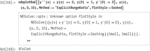
When writing or working with functions that use options, keep in mind that Mathematica’s convention is to give precedence to options that appear earlier in the list. So if two options conflict, the first wins.