You want to perform computations that take as input information about the chemical elements. You may also want to create visual displays of this information for reference or classroom use.

You can list the names of all the elements using ElementData[] or the name of the nth element using ElementData[n].

In[1]:=  ElementData[]
Out[1]=  {Hydrogen, Helium, Lithium, Beryllium, Boron, Carbon, Nitrogen, Oxygen,
          Fluorine, Neon, Sodium, Magnesium, Aluminum, Silicon, Phosphorus, Sulfur,
          Chlorine, Argon, Potassium, Calcium, Scandium, Titanium, Vanadium,
          Chromium, Manganese, Iron, Cobalt, Nickel, Copper, Zinc, Gallium,
          Germanium, Arsenic, Selenium, Bromine, Krypton, Rubidium, Strontium,
          Yttrium, Zirconium, Niobium, Molybdenum, Technetium, Ruthenium, Rhodium,
          Palladium, Silver, Cadmium, Indium, Tin, Antimony, Tellurium, Iodine,
          Xenon, Cesium, Barium, Lanthanum, Cerium, Praseodymium, Neodymium,
          Promethium, Samarium, Europium, Gadolinium, Terbium, Dysprosium,
          Holmium, Erbium, Thulium, Ytterbium, Lutetium, Hafnium, Tantalum,
          Tungsten, Rhenium, Osmium, Iridium, Platinum, Gold, Mercury, Thallium,
          Lead, Bismuth, Polonium, Astatine, Radon, Francium, Radium, Actinium,
          Thorium, Protactinium, Uranium, Neptunium, Plutonium, Americium,
          Curium, Berkelium, Californium, Einsteinium, Fermium, Mendelevium,
          Nobelium, Lawrencium, Rutherfordium, Dubnium, Seaborgium, Bohrium,
          Hassium, Meitnerium, Darmstadtium, Roentgenium, Ununbium, Ununtrium,
          Ununquadium, Ununpentium, Ununhexium, Ununseptium, Ununoctium}

In[2]:=  ElementData[1]
Out[2]=  Hydrogen

Mathematica will return properties of an element if given its number and the name of the property.

In[3]:=  Row[{ElementData[1], ElementData[1, "AtomicNumber"],
           ElementData[1, "AtomicWeight"], ElementData[1, "Phase"]}, "	"]
Out[3]=  Hydrogen    1    1.00794    Gas

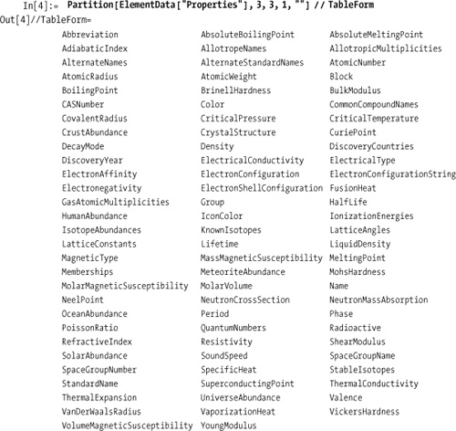
You can see from the list of all properties that Mathematica has a comprehensive database of elemental data. Be aware that CommonCompoundNames will pull in a lot of data if you use it with a common element like hydrogen.

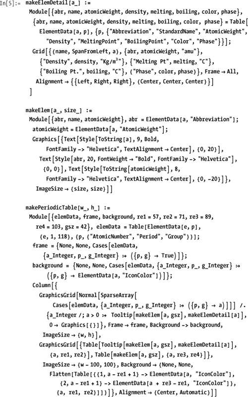
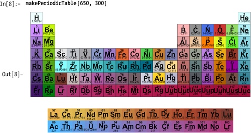
The most obvious application of ElementData is to create a periodic table. The ElementData documentation shows code for a simple table. Here I show a more ambitious one, complete with Tooltip.

You want to perform computations that take as input information about the chemical compounds. You may also want to create visual displays of this information for reference or classroom use.

ChemicalData is a curated data source. You can request chemical information by common names, registry numbers, IUPAC-like names, or structure strings.

The list of properties of chemical compounds is quite impressive. The table below lists a random subset of the full list of 101 properties.

   In[14]:=  Partition[Sort[RandomSample[ChemicalData["Properties"], 30]], 3] //
             TableForm
Out[14]//TableForm=
             AcidityConstant      BoilingPoint            CHStructureDiagram
             CIDNumber            CompoundFormulaDisplay   CriticalPressure
             CriticalTemperature FlashPointFahrenheit     FormattedName
             HildebrandSolubility IUPACName               MDLNumber
             MeltingPoint         NFPAHazards             NFPAHealthRating
             NFPALabel            NonStandardIsotopeCount NonStandardIsotopeNumbers
             PartitionCoefficient Phase                   Resistivity
             RotatableBondCount   SideChainAcidityConstant SpaceFillingMoleculePlot
             StructureDiagram     TautomerCount           TopologicalPolarSurfaceArea
             VaporPressureTorr    VertexTypes             Viscosity

At the time of this writing, Mathematica has curated data on over 34,300 compounds, subdivided into 67 classes.

In[15]:=  Length[ChemicalData[]]
Out[15]=  34336

In[16]:=  ChemicalData["Classes"]
Out[16]=  {AcidAnhydrides, AcidHalides, Acids, Alcohols, Aldehydes, Alkanes,
           Alkenes, Alkynes, Alloys, Amides, Amines, AminoAcidDerivatives,
           AminoAcids, Arenes, Aromatic, Bases, Brominated, Carbohydrates,
           CarboxylicAcids, Catalysts, Cations, Ceramics, Chiral, Chlorinated,
           Dendrimers, Esters, Ethers, Fluorinated, Furans, Gases, Halogenated,
           HeavyMolecules, Heterocyclic, Hydrides, Hydrocarbons, Imidazoles,
           Indoles, Inorganic, Iodinated, IonicLiquids, Ketones, Ligands,
           Lipids, Liquids, MetalCarbonyls, Monomers, Nanomaterials, Nitriles,
           Organic, Organometallic, Oxides, Phenols, Piperazines, Piperidines,
           Polymers, Pyrazoles, Pyridines, Pyrimidines, Quinolines, Salts, Solids,
           Solvents, Sulfides, SyntheticElements, Thiazoles, Thiols, Thiophenes}

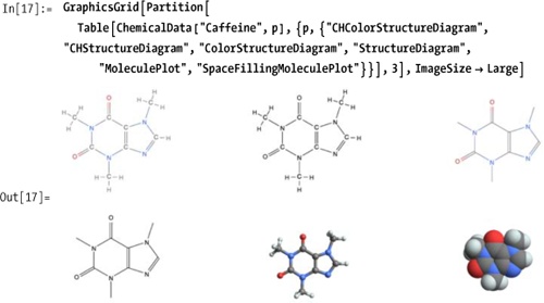
There are six kinds of structural diagrams that can be used to visualize these compounds. Here, for example, are representations for what may be one of your favorites, for better or worse—caffeine.

You can use the data to analyze relationships between properties. Here I show a plot of inverse vapor pressure to boiling point for all liquids with a Tooltip around each point so outliers are easy to identify. Cases is used to filter out any MissingData entries.

You want to perform computations that take as input information about the elementary particles. You may also want to create visual displays of this information for reference or classroom use.

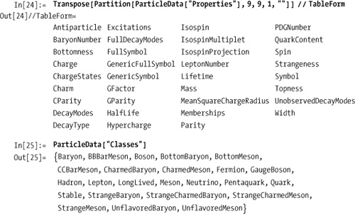
In[19]:= ParticleData["Classes"]
Out[19]= {Baryon, BBBarMeson, Boson, BottomBaryon, BottomMeson,
          CCBarMeson, CharmedBaryon, CharmedMeson, Fermion, GaugeBoson,
          Hadron, Lepton, LongLived, Meson, Neutrino, Pentaquark, Quark,
          Stable, StrangeBaryon, StrangeCharmedBaryon, StrangeCharmedMeson,
          StrangeMeson, UnflavoredBaryon, UnflavoredMeson}

It is easy to create functions that generate tables of particle information. The function particleTable accepts a list of one or more class memberships (e.g., Baryon, LongLived, and others from ParticleData["Classes"]) and a list of properties to use as columns. The helper function particleData reformats "QuarkContent" into a more concise representation. You will often want to filter out entries that are missing since there is only partial data available for exotic particles.

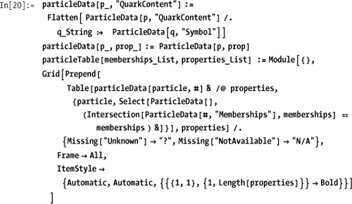
Create a table of long-lived baryons. A baryon is a particle made of three quarks, and long-lived refers to particles whose lifetime is greater than 10^–20 seconds.

The list of properties available in particle data are as follows:

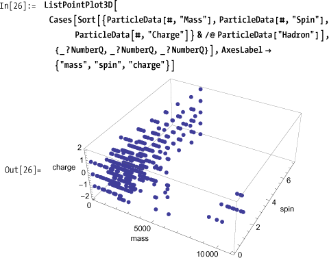
A scatter plot of mass versus spin versus charge shows large voids where there are no known particles (or where the values are unknown).

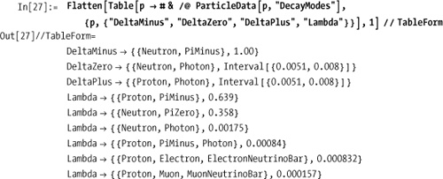
DecayModes and FullDecayModes list the ways the particle can decay; FullDecayModes also lists those predicted by theory but not observed in detectors. The number (or interval) display with the decay mode is the branch ratio.

You want to use Mathematica’s pattern matching and computational capabilities to develop bioinformatics applications. GenomeData and ProteinData provide the raw materials for this application.

Get the first 100 nucleobases (or, simply, bases) on the male X chromosome.

Get the first 10 proteins known to Mathematica and show number of amino acids in its sequence.

      In[29]:=  {#, ProteinData [#, "SequenceLength"]} & /@
                  Take[ProteinData[], 10]  // TableForm
Out[29]//TableForm=
             A1BG      495
             A2M       1474
             NAT1      290
             NAT2      290
             SERPINA3  423
             AADAC     399
             AAMP      434
             AANAT     207
             AARS      968
             ABAT      500

Find five other chromosomes that have sequences that match the first 50 bases of chromosome-1 in the human genome. Strands of the chromosome are indicated as 1 or -1.

In[30]:=  GenomeLookup[GenomeData[{"Chromosome1", {1,50}}], 5]
Out[30]=  {{{Chromosome1, 1}, {1, 50}}, {{Chromosome1, 1}, {7, 56}},
           {{Chromosome1, 1}, {13, 62}}, {{Chromosome3, -1}, {116621, 116670}},
           {{Chromosome3, -1}, {116615, 116664}}}

At the time of writing, Mathematica has data on 27,479 proteins and 39,920 genes.

In[31]:=  {Length[ProteinData[]], Length[GenomeData[]]}
Out[31]=  {27479, 39 920}

The following is a list of properties of the proteins. This data is somewhat incomplete: some of the values are not known or have not been updated in Wolfram’s database. The good news is that it improves over time, so there is likely more data when you’re reading this than when I wrote it. Notice how this sample is ordered in columns, whereas prior recipes showed similar lists in rows. All you need is Transpose and a bit of math to get the desired number of columns.

In[32]:=  Module[{props = ProteinData["Properties"]},
            With[{nCols = Ceiling[Length[props]/3]},
             Transpose[Partition[props, nCols, nCols, 1, "" ]]]]//TableForm
Out[32]//TableForm=
             AdditionalAtomPositions  DNACodingSequence        MolecularWeight
             AdditionalAtomTypes      DNACodingSequenceLength  MoleculePlot
             AtomPositions            DomainIDs                Name
             AtomRoles                DomainPositions          NCBIAccessions
             AtomTypes                Domains                  PDBIDList
             BiologicalProcesses      Gene                     PrimaryPDBID
             CellularComponents       GeneID                   SecondaryStructureRules
             ChainLabels              GyrationRadius           Sequence
             ChainSequences           Memberships              SequenceLength
             DihedralAngles           MolecularFunctions       StandardName

One property that is sparsely populated is MoleculePlot. At the time of writing, the only protein beginning with "ATP" that has a MolecularPlot is ATP7BIsoformA.

GenomeData likewise contains a wealth of information. Here I show the properties available.

In[34]:=  Module[{props = GenomeData["Properties"]},
            With[{nCols = Ceiling[Length[props]/3]},
             Transpose[Partition[props, nCols, nCols, 1, ""]]]]//TableForm
Out[34]//TableForm=
             AlternateNames          GBandStainingLevels    Orientation
             AlternateStandardNames  GenBankIndices         ProteinGenBankIndices
             BiologicalProcesses     GeneID                 ProteinNames
             CellularComponents      GeneOntologyIDs        ProteinNCBIAccessions
             Chromosome              GeneType               ProteinStandardNames
             CodingSequenceLists     InteractingGenes       PubMedIDs
             CodingSequencePositions IntronSequences        SequenceLength
             CodingSequences         LocusList              StandardName
             ExonSequences           LocusString            TranscriptGenBankIndices
             FullSequence            Memberships            TranscriptNCBIAccessions
             FullSequencePosition    MIMNumbers             UniProtAccessions
             GBandLocusStrings       MolecularFunctions     UnsequencedPositions
             GBandScaledPositions    Name                   UTRSequences
             GBandStainingCodes      NCBIAccessions

   In[35]:=  GenomeData["ACOT9", "ProteinNames"]
   Out[35]=  {acyl-Coenzyme A thioesterase 2, mitochondrial isoform a,
              acyl-Coenzyme A thioesterase 2, mitochondrial isoform b}
   In[36]:=  GenomeData["ACOT9", "Memberships"]
   Out[36]=  {ChromosomeXGenes, Genes, Hydrolase,
              Mitochondrion, ProteinBinding, ProteinCoding}
   In[37]:=  GenomeData["ACOT9", "CellularComponents"]
   Out[37]=  {Mitochondrion}
   In[38]:=   GenomeData["ACOT9", "MolecularFunctions"]
   Out[38]=  {AcetylCoAHydrolaseActivity,
              CarboxylesteraseActivity, HydrolaseActivity, ProteinBinding}

You want to model a dynamic system consisting of populations of predators and prey to see how population levels evolve over time.

Consider a population of rabbits (prey) and foxes (predators) with a specific growth rate for rabbits G and carrying capacity of their environment K. The population dynamics can be modeled by a pair of difference equations. See the Discussion section for more insight into the form of these equations and the meaning of the constants.

NestList presents one possible solution for deriving the dynamics of the population over time from an initial starting point.

This shows the rabbit population doing what rabbits do for many generations as the fox population slowly increases due to the increasing food supply. An inflection point is reached, and the fox population begins to take off with a resulting collapse in the rabbit population. Eventually the system reaches equilibrium.

The equation for rabbits assumes that rabbits follow the logistic model of exponential growth limited by the carrying capacity of the environment and then subtracts a term proportional to the number of rabbits and foxes where the constant 0.0001 reflects the efficiency of the predators. The equation for foxes assumes that the fox population is proportional to the ability to catch rabbits (same term from first equation) minus some natural death rate (here 2 percent of the population).

NestList provides a very simple solution to this model, but it is not the best choice if, due to efficiency, you want to create an interactive model using Manipulate. Luckily, Mathematica 7 has new capabilities for discrete math that provide an alternate solution path. RecurrenceTable is a new function that will generate the list of solutions of specified length given a recurrence relation.

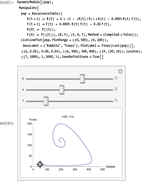
This interactive model allows you to position the locator at the initial population levels for rabbits and foxes and allows you to adjust the growth rate, carrying capacity, and number of iterations. The plot title displays the end value of rabbits and foxes.

More elaborate predator-prey models can be found at the Wolfram Demonstration Project: http://bit.ly/mUVGS and http://bit.ly/21GfLm.

You want to compute mass, center of mass, and moment of inertia as a prerequisite to solving dynamical problems involving rigid bodies.

The basic equation for computing the center of mass given a collection of discrete point masses is

where cm_i is the center of mass of each point and m_i is its mass. The numerator of this equation is called the first moment. Another name for the center of mass is the centroid.

In[43]:=  centerMass[particles_] := Module[{totalMass, firstMoment},
            {firstMoment, totalMass } =
             Sum[{mass @ particles[[i]] centroid @ particles[[i]],
               mass @ particles[[i]]}, {i, Length[particles]}];
            firstMoment/ totalMass]

In[44]:=  mass@car = 1000.;
          centroid @ car = {100, 100};
          mass @ driver = 86.;
          centroid@driver = {103, 101} ;
          mass@fuel = 14.2;
          centroid @ fuel = {93, 100};
          centerMass[{car, driver, fuel}]
Out[50]=  {100.144, 100.078}

The solution is fairly elementary from a physical point of view, but it may look a bit mysterious from a Mathematica coding point of view. The solution is coded using Mathematica’s prefix notion. Recall that f@x is prefix notation for f[x]. This notation is appealing for modeling problems because it is concise and readable (simply replace the @ with "of" as you read the code). Notice how I use the same notation with the problem objects car, driver, and fuel.

Now suppose this notation does not appeal to you; perhaps you like to model the physical objects as lists or some other notation like object[{mass,centroid}]. Does this mean you need to reimplement the centerMass function? Not at all. Simply define the function’s mass and centroid for your preferred representation, and you are all set.

In[51]:=  mass[object[{m_,__}]] := m

In[52]:=  centroid[object[{_, c_,__}]] := c

In[53]:=  centerMass[{object[{1000, {100, 100}}],
            object[{86, {103, 101}}], object[{14.2, {93, 100}}]}]
Out[53]=  {100.144, 100.078}

Another important property of rigid bodies is the mass moment of inertia about an axis. These values are important when solving problems involving rotation of the body. The general equation for the mass moment of inertia involves integration over infinitesimal point masses that make up the body, but in practice problems, equations for known geometries are typically used. One way to approach this in Mathematica is to use a property called shape and rely on pattern matching to select the appropriate formula. Each of these functions returns a list in the form {Ixx, Iyy, Izz}, giving the moment of inertia about the x-, y-, and z-axis, respectively.

In[1]:=  massMomentOfInertia[o_] /; shape@o == "circularCylinder" :=
          Module[{i1, i2},
           i1 = ((mass@o radius@o^2)/4) + ((mass@o length @o ^2)/12);
           i2 = ((mass@o radius@o^2)/2);
             {i1, i1, i2} ]
         massMomentOfInertia[o_] /; shape@o == "circularCylindricalShell" :=
          Module[{i1, i2},
           i1 = ((mass@o radius@o^2)/2) + ((mass@o length @o ^2)/12);
           i2 = ((mass@o radius@oA2));
            {i1, i1, i2} ]

         massMomentOfInertia[o_] /; shape@o == "rectangularCylinder" :=
          Module [{ixx, iyy, izz},
           ixx = ((mass@o (height@o + length@o) ^2)/12);
           iyy = ((mass@o (width@o + length@o) ^2)/12);
           izz = ((mass@o (width@o + height@o) ^2)/12);
            {ixx, iyy, izz} ]
         massMomentOfInertia[o_] /; shape@o == "sphere" := Module[{i},
           i = (mass@o (2 radius@o ^2)/5);
            {i, i, i} ]
         massMomentOfInertia[o_] /; shape@o == "sphericalShell" := Module[{i},
           i = (mass@o (2 radius@o A2) /3);
            {i, i, i} ]

In[59]:=  shape@car = "rectangularCylinder";
          length@car = 4.73;
          width@car = 1.83;
          height@car = 1.25;

In[63]:=  massMomentOfInertia[car]
Out[63]=  {2980.03, 3586.13, 790.533}

In[64]:=  shape@car = "circularCylindricalShell";
          radius@car = 1.83;

In[66]:=  massMomentOfInertia[car]
Out[66]=  {3538.86, 3538.86, 3348.9}

You want to demonstrate standard problems in kinematics, like those you typically find in first-year physics studies.

The basic equations of kinematics are as follows.

In[67]:=  acceleration1[deltaT_, v1_, v2_] := (v2 - v1) / deltaT
          acceleration2[deltaT_, v1_, deltaS_] :=
           2 (deltaS - v1 deltaT) / (deltaT^2)
          acceleration3[v1_, v2_, deltaS_] := (v2^2 - v1^2) / (2 deltaS)
          distance[a_, v1_, deltaT] := (adeltaT^2 / 2) + v1 deltaT
          distance1[a_, v1_, v2_] := (v2^2 - v1^2) / (2 a)
          distance2[deltaT, v1_, v2_] := (deltaT / 2) (v1 + v2)
          time1[a_, v1_, v2_] := (v2 - v1) / a
          time2[a_, v1_, deltaS] := (Sqrt[v1^2 + 2 + 2adeltaS] - v1) / a
          time3[v1_, v2_, deltaS] := (2 deltaS) / (v1 + v2)
          velocity1[a_, v2_, deltaT_] := v2 - a deltaT
          velocity2[a_, deltaS_, deltaT_] := (deltaS/ deltaT) - (a deltaT/ 2)
          velocity3[a_, v2_, deltaS_] := Sqrt[v2^2 - 2 a deltaS]

Given these equations, you can solve a variety of problems. For example, how far will a bullet drop if shot horizontally from a rifle at a target 500 m away if the initial velocity is 800 m/s? Ignore drag, wind, and other factors.

First, compute how long the bullet remains in flight before hitting the target by taking the initial and final velocity to be the same.

In[79]:=  timeTraveled  = time3[800, 800, 500] // N
Out[79]=  0.625

Given the acceleration due to gravity is 9.8 m/s², compute the distance dropped by setting the initial vertical velocity component to zero.

In[80]:=  distanceDropped  = distance[9.8, 0, timeTraveled]
Out[80]=  1.91406

The bullet drops almost 2 meters.

The solution works out a simple problem by working first in the x direction and then plugging the results into an equation in the y direction. In more complex problems, it is often necessary to use vectors to capture the velocity components in the x, y, and z directions. Consider a game or simulation involving a movable cannon and a movable target of varying size.

Imagine the cannon is fixed to the side of a fortress such that the vertical height (z direction in this example) is variable but the x and y position is fixed. The length, angle of elevation (alpha), left-right angle (gamma), and muzzle velocities are also variable. You require a function that gives the locus of points traversed by the shell given the cannon settings and the time of flight. Here we use Select to filter the points above ground level (positive in the z direction). The function returns a list of values of the form {{x1,y1,z1,t1}, ..., {xn,yn,zn,tn}}, where each entry is the position of the shell at the specified time. Chop is used only to replace numbers close to zero by zero. Note that in each dimension, the basic kinematic equations are in play, but since the inputs are in terms of angles, some basic trigonometry is needed to get the separate x, y, and z components. Velocity is constant in the x-y plane (we are still ignoring drag), and the z-axis uses the initial velocity component and the fall of the shell due to gravity.

You can also create a function that computes the instantaneous velocity components at a specified time.

In[82]:=  velocity[velocity_, alpha_, gamma_, t_] :=
           With[{g = 9.8},
            Chop[
            If[t > 0,
             {velocity * Cos[alpha * Pi / 2],
              velocity * Cos[gamma * Pi],
              velocity Sin[alpha * Pi/ 2] - g t}, {0., 0., 0.}]
           ]
          ]

Since the plan is to create a simulation, you need a function that figures out when the shell intersects with the target. For simplicity, assume the shape of the target is a box.

You can set the simulation up inside of a Manipulate so that you can play around with all the variables.

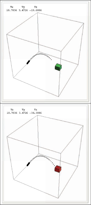
The initial output of the Manipulate is shown in Out[85] above. The path of the bullet is displayed up until the point in time specified by the time control, so the box turns red after it is hit by a shell. The instantaneous velocity of the shell is displayed for the current value of time. The Vz will be negative when the shell is falling. Figure 13-1 shows two frames from the Manipulate, at a time before impact and a time after.

David M. Bourg’s Physics for Game Developers (O’Reilly) has an example of the cannon problem where wind drag is introduced. Keep in mind that the author uses the y-axis as the vertical whereas the code in this recipe uses the z-axis.

Mathematical Methods Using Mathematica by Sadri Hassani (Springer) has solutions to similar problems using differential equations which consider drag, curvature of the earth, and nonconstant acceleration at large distances from the earth’s surface (see Chapter 6).

Figure 13-1. Two frames from the cannon simulation

You want to compute the normal modes for a system of identical masses connected by identical springs. Normal modes are natural or resonant frequencies of the entire system. The system this recipe considers consists of n>1 masses connected by n-1 springs on a frictionless surface. Figure 13-2 shows an example for n=3.

Figure 13-2. Coupled masses

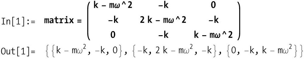
Here I state, without proof (refer to See Also section), that these systems take the form of n simultaneous linear equations whose matrix representation is tridiagonal. That is a matrix with nonzero entries along the main diagonal and adjacent minor diagonals and zero entries in all other elements. The corner entries of the main diagonal are special since they represent masses that are free on one side and take the form k - m*ω^2, where k is the spring constant, m is the mass, and ω is the angular frequency. The off corner entries represent the masses with springs on both sides and take the form 2*k - m*ω^2. The minor diagonals are all -k. Here I solve the three mass problems, and in the discussion, I show how to create a general solver for the n mass case.

Nontrivial solutions to this system leave the matrix as noninvertible; hence, the determinant is zero. Use Solve to find the frequencies in terms of k.

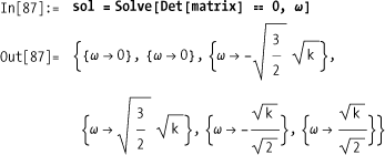
You don’t care about the solutions with negative or zero frequencies, so you can filter these out to obtain two physically interesting resonant frequencies.

Given the frequencies, you can solve the system to get the amplitudes. The first solution gives al == a3 and a2 == -2a1, with the alternative of k == 0 being physically uninteresting. This solution has the outer masses moving in unison in the same direction while the inner mass compensates by moving in the opposite direction with twice the amplitude.

In[89]:=  Reduce[Dot[(matrix /. sol[[1]]), {a1,a2,a3}] == 0, {a1,a2,a3}]
Out[89]= (a2 ==-2a1&&a3 = al) || k = 0

The second solution gives a2 == 0 and a3 == -al with the alternative of k == 0 being physically uninteresting. This is a solution with the center mass at rest and the outer masses moving toward and then away from the center.

In[90]:=  Reduce[Dot[(matrix /. sol[[2]]), {a1,a2,a3}] == 0, {a1,a2,a3}]
Out[90]=  (a2 = 0&&a3 == -al) || k = 0

To solve the general n-mass system, we need a way to synthesize a tridiagonal matrix of the proper form. For this, SparseArray and Band are just what the doctor ordered. When using sparse matrix, rules that come earlier override rules that come later. This works to your favor because it allows the case where n == 2 to be handled without any conditional logic stemming from the fact that there are no 2*k - m*ω^2 terms when n == 2.

For the general solution, you want to use NSolve with specific values of m and k because roots of polynomials with degree greater than five are likely to give Solve trouble. Here I solve a 10-mass system with k == 1 and m == 1. Chop is used to remove residual imaginary values and Cases filters out zero and negative solutions because they are physically uninteresting.

You can find derivations of the systems solved in this recipe in many advanced physics and linear algebra books. In particular, Mathematical Methods Using Mathematica by Sadri Hassani provides a nice mix of practical physics and Mathematica techniques, although the most recent edition is written for versions of Mathematica prior to 6 and therefore does not always indicate the best technique to use for current versions.

You want to model the dynamics of a vibrating string after it is released from a particular deformation.

This solution is a particular solution to the one-dimensional wave equation D[u[x,t], {x,2}] == c^2 D[u[x,t],{t,2}] where u[x,t] gives the position of the string at point x and time t. The general solution to the wave equation can be obtained using DSolve.

The general solution is not very helpful because it is specified in terms of two unknown functions, C[1] and C[2]. In theory, you could specify boundary conditions and initial conditions, but DSolve is very limited in its ability to find solutions to partial differential equations. This problem is better handled numerically with NDSolve.

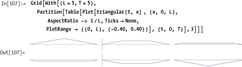
First we need a specification for the shape of the string at t = 0. For simplicity, I’ll use the Sin function that will give a width of L units. Here I use Plot to show the initial defection of the string.

To use NDSolve to model the vibrating string, you must provide initial and boundary conditions. The initial condition states that u[0,x] = string[x]. In other words, at the start, the string has the position depicted previously. You must also specify the initial velocity of the string, which is the first derivative with respect to time. The obvious choice for initial velocity is zero. Using input form, this would be entered as Derivative[1, 0][u][0, x] == 0. This operator notation was explained in 11.4 Differentiating Functions. The two boundary conditions specify that the ends of the string are anchored at position 0 and L, u[t, 0] == 0, and u[t, L] == 0.

Although DSolve can deal with some partial differential equations (PDEs), it is limited in its ability to derive specific solutions given initial and boundary conditions. Therefore, it is better to use NDSolve on PDEs, as I’ve done in the solution. However, it is not difficult to pose problems that NDSolve will have a hard time with and ultimately fail to solve. Consider trying to solve the wave equation with an initial position that contains a discontinuity.

If you try to use string2 in the solution shown in In[99] above, it will likely run for a very long time, consuming memory and finally failing. However, this situation is not entirely hopeless. One technique is to produce an approximation to string2 using Fourier series. Using Fourier series, I obtained the following Sin expansion, called sinString2:

In[102]:=  sinString2[x_] = 0.285325252629769` Sin[(Pi*x)/5] -
              0.033193742967516204` Sin[(3*Pi*x)/5] +
              0.013117204588138661` Sin[πx] - 0.007723288156504195`
               Sin[(7*Pi*x)/5] + 0.005695145921372713` Sin[(9*Pi*x)/5] -
              0.004945365736699312` Sin[(11*Pi*x)/5];

Below I plot both functions to demonstrate how closely sinString2 approximates string2 while smoothing out the discontinuity at the apex.

There is an exact solution to the triangular wave, although it isn’t derived here (refer to the See Also section). It is given by this infinite sum, which Mathematica can solve using a special function LerchPhi. This solution is too complex to use in an animation, but you can use it to verify that the approximate solution is quite good.

Plotting a few snapshots of the exact solution over time tells us that the approximate solution is more than adequate and, in some sense, superior because it is far less computationally intense.

There are many ways to approach the solution to the wave equation. When this problem is solved by hand, separation of variables is often employed. See Advanced Engineering Mathematics by Erwin Kreyszig (John Wiley) for a step-by-step example. Warning: this book is not a Mathematica reference, but the problems are worked out in enough detail that you can easily see your way to creating your own Mathematica-based solutions.

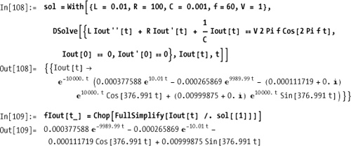
You want to understand how electrical circuits consisting of resistors, capacitors, and inductors behave.

The differential equation governing an RLC circuit is L I'' + R I' + I/C = E(t), where I is current, L is inductance, R is resistance, C is capacitance, and E(t) is the electromotive force (commonly known as voltage). Modeling the system means understanding how the current varies as you drive the system with a particular timing varying voltage. Let’s consider a common sinusoidal voltage and solve the system assuming that the charge and current are zero at t=0. Setting the problem up with the context of a With allows you to solve the problem for different values of inductance, capacitance, resistance, frequency, and voltage.

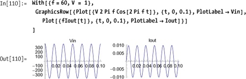
By plotting the input voltage and output current, you can see they have the same basic shape and frequency except for a phase shift.

A more interesting example uses a nonsinusoidal wave, such as a triangular wave. Conveniently, Mathematica 7 has a function TriangleWave[t] that suits our purpose.

However, the discontinuities in this waveform throw DSolve for a loop. To work around this, represent the triangular wave by its Fourier series. This will give a very close approximation without the discontinuities at the extremes. This will allow you to use DSolve.

Notice how the RLC circuit responds to the triangular wave input by smoothing the current flow to an approximately sinusoidal form. As an exercise, you can try this same example using SquareWave, SawtoothWave, or other functions of your own design.

You want to build a model based on the finite element method (FEM). You want to organize the model in a manner that allows you to obtain the solution as well as other intermediate results and structural diagrams.

The FEM has a wide range of engineering applications. In this recipe, I will limit the discussion to structures composed of linear elements known as trusses. See the figure shown in the "Discussion" section. Here my focus will be on the organization of the solution within Mathematica rather than on the underlying theory. Therefore, all results will be present without derivation of the underlying mathematics. Please refer to the references in the See Also section.

To begin, you will need a means to represent the elements. I use a structure called linearElement that specifies two endpoints called nodes ({{x1, y1}, {x2, y2}}), an area, and a measure of stiffness called Young’s Modulus (YM).

linearElement[{{x1, y1}, {x2, y2}}, area, YM]

In addition, you need a means for specifying the x and y components of the force at each node.

force[{x, y}, fx, fy]

Furthermore, at each node there is a computed displacement in the x and y direction. The FEM literature uses the variable u for x displacements and v for y displacements Typically, each node is sequentially numbered, so you would have ul, vl, u2, v2, and so on. I will not use a sequential numbering here, bocuuso ouch node is uniquely identified by its coordinates, and given Mathematica’s liberal representation of variables, it is much more convenient to specify nodal displacements using coordinates.

u[x1, y1]
(*The displacement in the x direction at node {x1,y1}*)
v[x1, y1] (*The displacement in the y direction at node {x1,y1}*)

With these conventions established, I proceed by defining a series of helper functions that will be needed later. I provide a brief description of each function but, for brevity, defer more detail to the Discussion section.

Each element in the model is governed by a system of linear equations. The system is naturally represented by a symmetric matrix. The symmetry takes the form {{A,-A},{-A,A}} where A is a block matrix.

A location vector provides a means for locating the position of the local element matrices computed by linearElementMatrix within a larger global matrix that represents the system over all elements.

In[119]:=  assemblyLocationVector[linearElement[{n1_, n2_},__], allnodes_] :=
            Flatten[Position[allnodes, #]& /@ {u@@n1, v@@n1, u@@n2, v@@n2}]

This helper maps a node of the form {{x1,y1},{x2,y2}} to the corresponding force components {{fx1,fy1},{{fx2,fy2}}}. It does this by searching for the first match of the node within the list of forces and transforming it to the desired form.

In[120]:=  getExternalForces[{forcesforce}, node_] :=
            Cases[{forces}, force[node, fu_, fv_] :> {fu, fv}, 1, 1]

This helper extracts the unique set of nodes from the elements and places them in a canonical order, as defined by Union. This ordering is essential to the construction of a consistent system of equations. See the Discussion section for details.

In[121]:=  getNodes[{elementslinearElement}] :=
            Union[{elements} /. linearElement[{n1_, n2_},__] :> Sequence[n1, n2]]

This helper is used to construct a replacement rule for forces.

Construct a global vector of all forces using a set of nodes in canonical order.

In[123]:=  getForceVector[{forces__force}, nodes_] :=
            Flatten[getExternalForces[{forces},  #]& /@ nodes]

Assemble the global matrix that defines the system of equations over all elements using the local matrices for individual elements and the location vectors that define the position of the local matrices with the global matrix. Note that the global matrix is obtained by summing the local matrices into the appropriate positions within the global matrix. In other words, think of each member of locationVectors as specifying a submatrix within the global matrix for which the corresponding member of localMatrices is added.

In[124]:=  assembleGlobalMatrix[localMatricies_,
             locationVectors_, numElements_, dimension_] :=
            Module[{g},
             g = Table[0, {dimension}, {dimension}] ;
             Do[g[[locationVectors[[i]], locationVectors[[i]] ]] +=
               localMatricies[[i]], {i, 1, numElements}] ;
             g
            ]

A model consists of a collection of connected elements, the external forces applied to the structure at one or more nodes, and the boundary conditions that typically manifest as points where a node is anchored, rendered immobile in the x, y, or both directions. Here I organize a solution in the spirit of LinearModelFit covered in Chapter 12. That is, I construct an object called a TrussModel, the function of which is to organize the underlying data and then use that object as the target for requests for certain properties relevant to the FEM. As of Mathematica 6 and particularly in Mathematica 7, this object-based methodology has emerged as a design pattern for organizing solutions that involve large quantities of data or collections of related functionality.

To proceed in this manner, you need a function for creating the TrussModel and a Format for displaying it. The Format is syntactic sugar that hides the details of the TrussModel, which could be quite large.

In[125]:=  createTrussModel[{elementslinearElement},
             {forces___force}, boundaryNodes_] :  =
           Module[{localMatrices, nodes, nodalVar, forceVec, locationVectors,
             degreesOfFreedom, globalMatrix, allForces, forceRules},
            nodes = getNodes[{elements}];
            nodalVar = Flatten[{u@@#, v@@#}&/@ nodes];
            localMatrices = linearElementMatrix /@ {elements};
            locationVectors = assemblyLocationVector [#, nodalVar] & /@ {elements};
            globalMatrix = assembleGlobalMatrix[localMatrices,
              locationVectors, Length[{elements}], Length[nodalVar]];
            degreesOfFreedom = Complement[Range[Length[nodalVar]],
              Flatten[Position[nodalVar, #]& /@ boundaryNodes]];
            allForces = force [#, 0, 0]& /@ nodes;
            forceRules = makeForceRule /@ {forces};
            allForces = allForces /. forceRules;
            forceVec = getForceVector[allForces, nodes];
            TrussModel[{elements}, boundaryNodes, localMatrices,
             globalMatrix, nodalVar, forceVec, degreesOfFreedom, forces]]

         Format[TrussModel[elements_, boundaryNodes_, __ ]] :=
          ToString[TrussModel[{Length[elements]}, {Length[boundaryNodes]}]]

The goal of a FEM analysis is to determine the behavior of the structure from the behavior of the elements. For a system of trusses, solve for the displacements at the joints, the axial forces, and axial stresses. Following the proposed methodology, these will be accessed as properties of the TrussModel.

The displacements property is implemented as a functional pattern associated with the TrussModel. This notation may look somewhat unusual but is quite natural from the standpoint of Mathematica’s design. It simply states that when you see a pattern consisting of a TrussModel and a literal argument, "displacements", replace it with the results of computing the displacements using data from the TrussModel.

In[127]:= TrussModel[_, _, _, globalMatrix_, nodalVars_,
             forceVec_, degreesOfFreedom_, ___]["displacements"] :=
           Flatten[Solve[Dot[globalMatrix[[degreesOfFreedom, degreesOfFreedom]],
               nodalVars[[degreesOfFreedom]]] ==
              forceVec[[degreesOfFreedom]], nodalVars[[degreesOfFreedom]]]]

As a matter of convenience, you can make a property the default property of the model by associating it with the invocation of the model with no arguments. Of course, thus far I have defined only one property, displacements, but it was my intent to make this the default. In the discussion I derive other properties of this model.

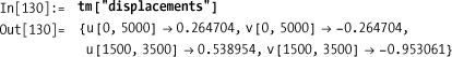
In[128]:=  TrussModel[model][] := TrussModel[model]["displacements"]

All this tedious preparation leads us to a solution that is very easy to use. Here is the TrussModel, depicted in Out[136] on Discussion. The example data is borrowed from a problem presented in Bhatti’s book (refer to the See Also section).

In[129]:=  tm = createTrussModel[
             {linearElement[{{0, 0}, {1500, 3500}}, 4000., 200*10^3],
              linearElement[{{1500, 3500}, {5000, 5000}}, 4000., 200*10^3],
              linearElement[{{0, 0}, {0, 5000}}, 3000., 200*10^3],
              linearElement[{{0, 5000}, {5000, 5000}}, 3000., 200*10^3],
              linearElement[{{0, 5000}, {1500, 3500}}, 2000., 70*10^3]},
             {force[{1500, 3500}, 0, -150000]},
             {u[0, 0], v[0, 0], u[5000, 5000], v[5000, 5000]}]
Out[129]=  TrussModel[{5}, {4}]

Now you can compute the nodal displacements at the nodes that are unsupported.

To complete the TrussModel, we need to define more properties. It is nice to have a visual aid to help diagnose problems in the setup of the model. A "diagram" property generates graphics. As before, I need to develop some helper functions to take care of certain tails. Each helper function has a placeholder for options (opts___), but to keep the implementation from getting any more complicated, I do not implement any options. You could add options to control the level of detail, for example, to include or suppress displacement arrows and labels. Other options might be pass-through options to Graphics.

The diagram uses a convention where supported nodes are filled-in points, whereas unsupported nodes are hollow circles with associated displacement arrows. It is possible that a node can be stationary in one direction but not the other. For example, a roller would be free to move in the x direction but not the y. Professional FEM software handles a much wider variety of boundary conditions, and standard icons are used in the industry to depict these. The goal here is simplicity over sophistication.

The function trussGraphicsNodes does most of the work of mapping the various types of nodes onto the specific graphics element. The complexity of the code is managed by judicious use of patterns and replacement rules. Some of the scaling and text placement was largely determined by trial and error, so you may need to tweak these settings for your own application or add additional code to help generalize the solution.

As before, once the infrastructure is in place, the diagram is easy to create by simply asking the model for the "diagram" property.

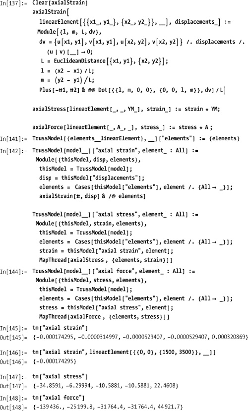
Other important properties are axialStrain, axialStress, and axialForce. These will be implemented to return all or specific values for a specified element.

There are many books and online resources that cover FEM. For example, the theory relevant to truss structures can be found at Jason Midkiff’s Virginia Tech science and engineering website: http://bit.ly/32BUq1 .

If you are looking for books with a Mathematica focus, look no further than Fundamental Finite Element Analysis and Applications: With Mathematica and Matlab Computations (John Wiley) and—if you are really into FEM— Advanced Topics in Finite Element Analysis of Structures: With Mathematica and MATLAB Computations (John Wiley), both by M. Asghar Bhutti. The code in these books is pre-version 6, but I found few incompatibilities.