I’ve been looking so long at these pictures of you that I almost believe that they’re real I’ve been living so long with my pictures of you that I almost believe that the pictures are all I can feel
—The Cure, "Pictures of You"
One of the features that places Mathematica in a class by itself
among similar computer-aided mathematics tools is its advanced graphics
capabilities. This chapter focuses on two-dimensional graphics.
Mathematica provides a variety of plotting functions with a versatile
set of options for customizing their display. The most common types of
2D graphic are the plot of a function and list plots of values. 6.1 Plotting Functions in Cartesian Coordinates covers Plot and 6.4 Plotting Data
covers ListPlot. Frequently you will
want to use other coordinate systems or scales. In two dimensions,
PolarPlot and ParametricPlot are often used as demonstrated
in 6.1 Plotting Functions in Cartesian Coordinates and 6.2 Plotting in Polar Coordinates.
True to its symbolic nature, Mathematica represents all graphics
as collections of graphics primitives and directives. Primitives include
objects such as Point and Line; directives provide styling information
such as Thickness and Hue. Mathematica allows you to work with the
low-level primitives (see 6.8 Displaying 2D Geometric Shapes), but most readers will be
interested in the higher-level functions like Plot and ListPlot, which generate graphics from
functions and data and display them. However, it is easy to demonstrate
that these functions generate primitives by specifying InputForm.
In[1]:=  ListPlot[{0, 1, 2, 3}] // InputForm
Out[1]//InputForm=
             Graphics[{Hue[0.67, 0.6, 0.6],
               Point[{{1., 0.}, {2., 1.}, {3., 2.}, {4., 3.}}]},
              {AspectRatio -> GoldenRatio^(-1), Axes -> True,
               AxesOrigin -> {0, Automatic},
               PlotRange -> Automatic, PlotRangeClipping -> True}]
This uniform representation allows graphics to be
manipulated programmatically, just like any Mathematica object, and
sometimes can be useful for generating custom effects. However, this
representation is not entirely at the lowest level, because graphics
constructs like axes are implicitly specified via options. To get to the
lowest level you can use the function FullGraphics. Here I use Short to suppress some of the details.
    In[2]:=  Short[InputForm[FullGraphics[ListPlot[{0, 1, 2, 3}]]], 10]
Out[2]//Short=
             Graphics[{{Hue[0.67, 0.6, 0.6], Point[{{1., 0.}, {2., 1.}, {3.,
               2.}, {4., 3.}}]}, {{GrayLevel[0.], AbsoluteThickness[0.25],
               Line[{{0.2, 0.}, {0.2, 0.010112712429686845}}]}, Text[0.2,
               {0.2, -0.02022542485937369}, {0., 1.}], {GrayLevel[0.],
               AbsoluteThickness[0.25], Line[{{0.4, 0.}, {0.4,
               0.010112712429686845}}]}, Text[0.4, {0.4, -0.02022542485937369},
               {0., 1.}], {GrayLevel[0.], AbsoluteThickness[0.25],
               Line[{{0.6000000000000001, 0.}, {0.6000000000000001,
               0.010112712429686845}}]}, Text[0.6000000000000001,
               {0.6000000000000001, -0.02022542485937369}, {0., 1.}],
               {GrayLevel[0.], AbsoluteThickness[0.25], Line[{{0.8, 0.}, {0.8,
               0.010112712429686845}}]}, <<41>>, {GrayLevel [0.], <<2>>},
               {GrayLevel[0.], AbsoluteThickness[0.125], Line[{{0., 0.9}, {0.00375,
               0.9}}]}, {GrayLevel[0.], AbsoluteThickness[0.125], Line[{{0.,
               0.9500000000000001}, {0.00375, 0.9500000000000001}}]}, {GrayLevel[0.],
               AbsoluteThickness[0.25], Line[{{0., 0.}, {0., 1.}}]}}}]
In the recipes that follow, I make frequent use of GraphicsRow, GraphicsColumn, and GraphicsGrid. These are handy for formatting
multiple graphics outputs across the page to make maximum use of both
horizontal and vertical space. Both GraphicsRow and GraphicsColumn take a list of graphics to
format, whereas GraphicsGrid takes a
matrix. To help generate these lists and matrices, I sometimes use
Table and Partition. These functions are simple enough
that I hope they do not detract from the intended lesson of the recipe.
6.6 Displaying Multiple Graphs in a Grid explains the use
of these gridlike formatting functions in detail.
The simplest solution is to use the Plot command with the range
of values to plot. Plot takes one or more functions of a single
variable and an iterator of the form {var, min, max}.

Plot has a wide variety of options for controlling the appearance of the plot. Here are the defaults.

When plotting two or more functions, you may want to
explicitly set the style of each plot’s lines. You can also suppress
one or both of the axes using Axes,
as I do in the second and fourth plots. You can label one or both of
the axes using AxesLabel and
control the format using LabelStyle.

PlotLabel is a handy
option for naming plots, especially when you display several plots at
a time.

You can add grid lines with an explicitly determined frequency or a frequency determined automatically by Mathematica.

Frame, FrameStyle, and FrameLabel let you annotate the graph with a
border and label. Note that FrameStyle and FrameLabel only have effect if Frame→True is also specified.

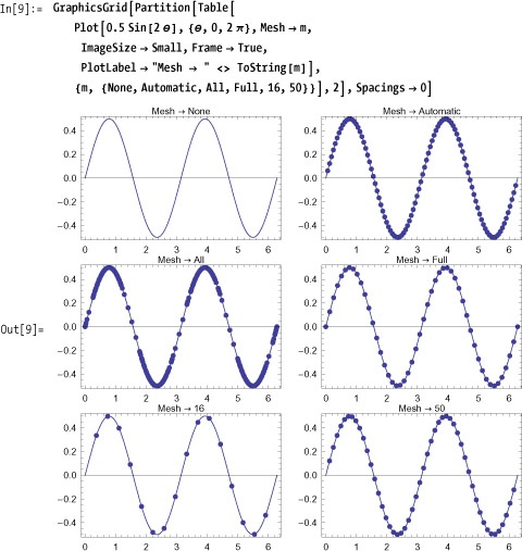
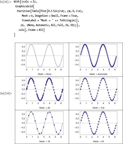
Mesh is an option that allows
you to highlight specific points in the plot. Mesh → All will highlight all points sampled
while plotting the graph, Mesh →
Full will use regularly spaced points. Mesh → n will use n equally spaced points. The behavior of
Mesh → Automatic will vary based on
the plotting primitive.
PlotRange is an
important option that controls what coordinates to include in the
plot. Automatic lets Mathematica
decide on the best choice, All
specifies all points actually plotted, and Full specifies the entire range. In
addition, you can supply explicit coordinates in the form {{xmin,xmax},{ymin,ymax}}.

AspectRatio controls
the ratio of height to width of the plot. The default value is
1/GoldenRatio (also known as
ϕ). A value of Automatic uses the coordinate values to
determine the aspect ratio.

Sometimes you want to emphasize an area on one side of
the curve or between two different curves. Filling can be set to Top to fill from the curve upward, Bottom to fill from the curve downward,
Axis to fill from the axis to the
curve, or to a numeric value to fill from the curve to that value in
either y direction.

FillingStyle allows
you to control the color and opacity of the filling. Specifying an
opacity is useful where regions of multiple functions overlap.

You can also use a special notation to fill the area
between two curves. In this notation, you refer to a curve by {i} where i is an integer referring to the
ith plot. You can then say something like
Filling → {i → {j}} to specify that
filling should be between plot i
and plot j. You can also override
the FillingStyle by including a
graphics directive, as in the example here.

6.2 Plotting in Polar Coordinates and 6.3 Creating Plots Parametrically demonstrate PolarPlot and ListPlot, which share most of the options of
Plot.
Use PolarPlot, which plots
the radius as the angle in polar coordinates varies counterclockwise
with 0 at the x-axis, π/2 at the y-axis, and so on.

As with Plot, you can
plot several functions simultaneously.

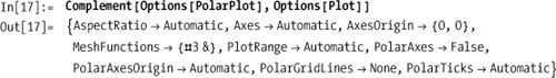
The options for PolarPlot are essentially the same as
Plot. One notable exception is the
absence of options related to Filling. Also note that AspectRatio is automatic by default, which
makes sense because symmetry is an essential aesthetic of polar
plots.
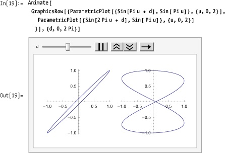
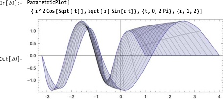
You want to create Lissajous curves and other parametric plots where points {fx[u], fy[u]} are plotted against a parameter u.
Here are some common Lissajous curves. Note how ParametricPlot takes a pair of functions in
the form of a list.

Here is an animation showing the effect of phase shifting on signals of frequency ratio 1:1 and 2:1.
You also use ParametricPlot
to create parametric surfaces. This introduces a second
parameter.
The 3D counterpart to ParametricPlot, ParametricPlot3D, is covered in 7.5 Creating 3D Contour Plots.
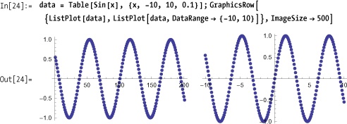
You want to graph data values that were captured outside Mathematica or previously computed within Mathematica.
Use ListPlot with either
lists of x values or lists of
(x,y) pairs. In this first plot, I generate the
y values but let the x
values derive from the iteration range. You can also explicitly
provide the x and y values
as a pair for each point plotted, as shown in the second ListPlot, which compares PrimePi to Prime.

ListPlot shares most
options with Plot; instead of repeating them here, I show only the
differences.

DataRange allows you to
specify minimum and maximum values for the x-axis. In the first plot,
the x-axis is assumed to be integer values.
InterpolationOrder is used
with Joined to control the way
lines drawn between points are interpolated. A value of 1 results in
straight lines; higher values result in smoothing, although for most
practical purposes, a value of 2 is sufficient.


When using Show to combine
plots, you can override options used in the individual graphs. For
example, you can override the position of axes, aspect ratio, and plot
range.

Show can be used to
combine arbitrary graphics. For example, you can give a graphic a
background image.

One of my favorite mathematical illustrations is
convergence through the iteration of a function (something I am sure
many of you have done by repeatedly pressing Cos
on a pocket calculator). Here, NestList performs 12 iterations. We
duplicate every two and flatten and partition into pairs with overhang
of 1 to yield the points for illustrating the convergence of the
starting point 1 to the solution of x ==
Cos[x].

Show uses the
following rules to combine plots:
Use the union of plot intervals.
Use the value of
Optionsfrom the first plot unless overridden byShow’s own options.
Use GraphicsGrid in
Mathematica 6 or GraphicsArray in
earlier versions. You can use tables to group several plots together,
but this gives you very little control of the layout of the images.
GraphicsGrid gives control of the
dimensions of the grid, the frame, spacing, dividers, and other
options. The dimensions of the grid are inferred from the dimensions
of the list of graphics passed as the first argument. You will find
Partition handy for converting a
linear list into the desired two-dimensional form.
In addition to GraphicsGrid, Mathematica provides GraphicsRow and GraphicsColumn, which are simpler to use for
laying out graphics horizontally or vertically. These layout functions
can be combined and nested to create more complex layouts. Here I
demonstrate using GraphicsRow to
show a GraphicsColumn next to
another GraphicsRow. Frames can be
drawn around the row or column (Frame→True) or additionally dividing all the
elements (Frame→All).

Use the PlotLegends` package
with the PlotLegend,
LegendPosition, and LegendSize options.

Legends use their own coordinate system, for which the
center of the graphic is at {0,0} and the inside is the scaled
bounding region {{-1,-1}, {1,1}}.
LegendPosition refers to the lower
left corner of the legend.
There are a variety of options for further tweaking the legend’s
appearance. You can turn off or control the offset of the drop shadow
(LegendShadow); control spacing of
various elements using LegendSpacing,
LegendTextSpace, LegendLabelSpace, and LegendBorderSpace; control the labels with
LegendTextDirection, LegendTextOffset,
        LegendSpacing,
and LegendTextSpace; and give the legend a label
with LegendLabel and LegendLabelSpace.
Notice the effect of LegendTextSpace, which is a bit
counterintuitive because it expresses the ratio of the text space to
the size of a key box so larger numbers actually shrink the legend.
LegendSpacing controls the space
around each key box on a scale where the box size is 1.

Sometimes you want to create a more customized legend.
In that case, consider Legend and
ShowLegend.
See the tutorial on the PlotLegends~ package at http://bit.ly/TYvfV .
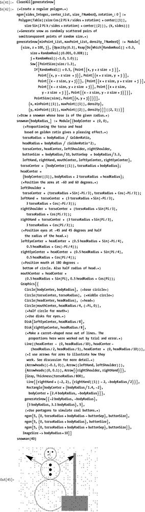
You want to create graphics that contain lines, squares, circles, and other geometric objects.
Mathematica has a versatile collection of graphics primitives:
Text, Polygon, Rectangle, Circle, Disk, Line,
        Point, Arrow, Raster,
and Point can be combined to create a variety of
2D drawings. Here I demonstrate a somewhat frivolous yet instructive
function that creates a snowman drawing using a broad sampling of the
available primitives. Included is a useful function, ngon, for creating regular polygons.
One of the keys to getting the most out of the graphics
primitives is to learn how to combine them with graphics directives.
Some directives are very specific, whereas others are quite general.
For example, Arrowheads applies
only to Arrow, whereas Red and Opacity apply to all primitives. A directive
will apply to all objects that follow it, subject to scoping created
by nesting objects within a list. For example, in the following
graphic, Red applies to Disk and Rectangle but not Line because the line is given a specific
color and thickness within its own scope.

Color directives can use named colors: Red, Green, Blue, Black, White, Gray, Cyan, Magenta,
Yellow, Brown, Orange, Pink, Purple, LightRed, LightGreen, LightBlue,
LightGray, LightCyan, LightMagenta, LightYellow, LightBrown,
LightOrange, LightPink, and LightPurple. You can also synthesize colors
using RGBColor or Hue, CMYKColor, GrayLevel, and Blend. In Mathematica 6 or later versions,
these directives can take opacity values in addition to values that
define the color or gray settings. Blend is also new to Mathematica 6.

Of course, you’ll need to try the code on your own to view the colors.
Thickness[r] is
specified relative to the total width of the graphic and, therefore,
scales with size changes. AbsoluteThickness[d] is specified in units
of printer points (1/72 inch) and does not scale. Thick and Thin are predefined versions (0.25 and 2,
respectively) of AbsoluteThickness.
Thickness directives apply to primitives that contain lines such as
Line, Polygon, Arrow, and the
like.

14.12 Visualizing Trees for Interest-Rate Sensitive Instruments applies Mathematica’s graphics primitives to the serious task of visualizing Hull-White trees, which are used in modeling interest-rate-sensitive securities.
13.11 Modeling Truss Structures Using the Finite Element Method shows an application in constructing finite element diagrams used in engineering.
Use Text with Style to specify FontFamily, FontSubstitutions, FontSize, FontWeight,
FontSlant, FontTracking, FontColor, and Background.

In this chapter, I demonstrate various plotting functions that contain options for adding labels to the entire graph, frames, and axes. These options can also be stylized.

The Style directive
was added into Mathematica 6 and is quite versatile. Style can add style options to both
Mathematica expressions and graphics.
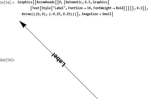
You want to create arrows with custom arrowheads, tails, and connecting lines for use in annotating graphics.

Arrowheads is quite
versatile. You can easily create double-ended arrows and arrows with
multiple arrowheads along the span.

You may consider using Arrowheads to label arrows, but Mathematica
does not treat such "arrowheads" specially, so you may get undesirable
effects.
A better option is to position the text by using
Rotate with Text or Inset or by using GraphPlot or related functions (see 4.6 Implementing Algorithms in Terms of Rules). The advantage
of Inset over manually positioned
Text is that you get auto-centering
if you don’t mind the label not being parallel to the arrow.

