The foundation of most data structures in Mathematica is the list. It is difficult to do much advanced work with Mathematica unless you are fluent in its functions for list processing. To this end, the initial recipes revolve around basic list processing. A list in Mathematica is constructed using the function List[elem1,elem2,...,elemN] or, more commonly, with curly brackets {elem1,elem2,...,elemN}. There is no restriction on the nature of these elements. They could be mixtures of numbers, strings, functions, other lists, or anything else Mathematica can represent (like graphic or sound data).

The first thing you need to know about lists is how to generate them. Table is the workhorse function for doing this. It has several variations that are most easily explained by example.

In addition to Table, Mathematica has several special-purpose list constructors: Range, Array, ConstantArray, DiagonalMatrix, and IdentityMatrix. These functions are less general than Table but are clearer and simpler to use when applicable. For example, consider IdentityMatrix and its Table equivalent.

Sometimes using a special-purpose list constructor is more verbose. Consider these equivalent ways of generating an array of ten 1s. Here, 1& is the function that always returns 1.

In[9]:=  Array[1&, 10] == ConstantArray[1, 10]
Out[9]=  True

Once you have one or more lists, you can compose new lists using functions like Append, Prepend, Insert, Join, and Riffle.

In[10]:=  list1 = Range[10]
Out[10]=  {1, 2, 3, 4, 5, 6, 7, 8, 9, 10}

In[11]:=  list2 = list1 ^ 2
Out[11]=  {1, 4, 9, 16, 25, 36, 49, 64, 81, 100}

In[12]:=  (*Add elements to the end.*)
          Append[list1, 11]
Out[12]=  {1, 2, 3, 4, 5, 6, 7, 8, 9, 10, 11}

In[13]:=  (*Add elements to the front.*)
          Prepend[list1, 0]
Out[13]=  {0, 1, 2, 3, 4, 5, 6, 7, 8, 9, 10}

In[14]:=  (*Insert elements at specific positions.*)
          Insert[list1, 3.5, 4]
Out[14]=  {1, 2, 3, 3.5, 4, 5, 6, 7, 8, 9, 10}

In[15]:=  (*Negative offsets to insert from the end*)
          Insert[list1, 3.5, -4]
Out[15]=  {1, 2, 3, 4, 5, 6, 7, 3.5, 8, 9, 10}

In[16]:=  (*You can insert at multiple positions {{i1},{i2},...,{iN}}.*)
          Insert[list1, 0, List /@ Range[2, Length[list1]]]
Out[16]=  {1, 0, 2, 0, 3, 0, 4, 0, 5, 0, 6, 0, 7, 0, 8, 0, 9, 0, 10}

In[17]:=  (*Join one or more lists.*)
          Join[list1, list2]
Out[17]=  {1, 2, 3, 4, 5, 6, 7, 8, 9, 10, 1, 4, 9, 16, 25, 36, 49, 64, 81, 100}

In[18]:=  (*Riffle is a function specifically designed to interleave elements.*)
          Riffle[list1, 0]
Out[18]=  {1, 0, 2, 0, 3, 0, 4, 0, 5, 0, 6, 0, 7, 0, 8, 0, 9, 0, 10}

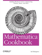
The flip side of building lists is taking them apart. Here you will use operations like Part, First, Last, Rest, Most, Take, Drop, Select, and Cases.

See Chapter 5 for more information on patterns.

You rearrange and restructure lists using functions such as Reverse, RotateLeft, RotateRight, Flatten, Partition, Transpose, and Sort

In[28]:=  Reverse[list1]
Out[28]=  {10, 9, 8, 7, 6, 5, 4, 3, 2, 1}

In[29]:=  RotateLeft[list1]
Out[29]=  {2, 3, 4, 5, 6, 7, 8, 9, 10, 1}

In[30]:=  RotateRight[list1]
Out[30]=  {10, 1, 2, 3, 4, 5, 6, 7, 8, 9}

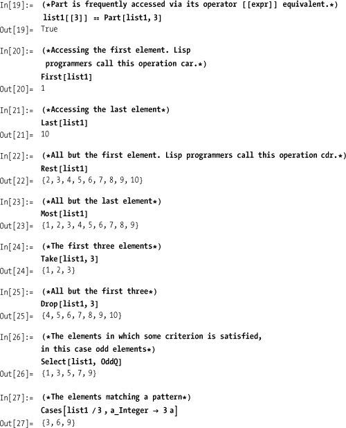
Partition and Flatten are very versatile functions for creating and removing structure. Flatten can be thought of as the inverse of Partition. Here, repeated partitioning using Nest converts a list to a binary tree.

Flatten can also take a level that tells it to flatten only up to that level.

Many of these functions have advanced features, so you should refer to the Mathematica documentation for each to understand their full capabilities. I will use these functions frequently throughout this book without further explanation, so if you are not already familiar with them, you should take some time to experiment on your own.

A set in Mathematica is nothing more than a list that is normalized to eliminate duplicates upon application of a set operation: Union, Intersection, or Complement. To determine duplicates, Mathematica uses an option called SameTest, which by default is the function SameQ or ===. The function Subsets constructs a list of all subsets. MemberQ is used to test membership, but this function is far more general, and I will revisit it in Chapter 4.

In[37]:=  Union[list1, list2]
Out[37]=  {1, 2, 3, 4, 5, 6, 7, 8, 9, 10, 16, 25, 36, 49, 64, 81, 100}

In[38]:=  Intersection[list1, list2]
Out[38]=  {1, 4, 9}

In[39]:=  (*Complement can be used with
           Intersection to implement Set Difference.*)
          Complement[list1, Intersection[list1, list2]]
Out[39]=  {2, 3, 5, 6, 7, 8, 10}

In[40]:=  Complement[list2, Intersection[list1, list2]]
Out[40]=  {16, 25, 36, 49, 64, 81, 100}

In[41]:=  (*Generating all subsets*)
          Subsets[{a, b, c}]
Out[41]=  {{}, {a}, {b}, {c}, {a, b}, {a, c}, {b, c}, {a, b, c}}

In[42]:=  MemberQ[list2, 4]
Out[42]=  True

A vector is also represented by a list, but Mathematica has a special representation called a SparseArray that can conserve space when a vector contains many zero entries (see 3.8 Using Sparse Arrays to Conserve Memory). Matrices and tensors are naturally represented as nested lists; these likewise can use SparseArrays.

Vector math is supported by the fact that most mathematical operations have the attribute Listable, meaning that the operations automatically thread over lists.

In[43]:=  (*Multiplication and subtraction of a vector by a scalar*)
          3 * list1 - 3
Out[43]=  {0, 3, 6, 9, 12, 15, 18, 21, 24, 27}

In[44]:=  (*Listable is the relevant property.*)
          Intersection[Flatten[Attributes[{Times, Plus, Minus, Divide, Power}]]]
Out[44]=  {Flat, Listable, NumericFunction,
           OneIdentity, Orderless, Protected, ReadProtected}

Same-sized vectors and matrices can also be added, multiplied, and so on, in an element-by-element fashion.

In[45]:=  Range[10] ^ Range[10, 1, -1]
Out[45]=  {1, 512, 6561, 16384, 15625, 7776, 2401, 512, 81, 10}

Vector-specific operations are also supported. Some of the more advanced operations are in a package called VectorAnalysis‘, including CrossProduct, Norm, Div, Grad, Curl, and about three dozen others. Use ?VectorAnalysis'* after loading the package to see the full list.

In[47]:=  u = {-1,0.5,1}; v = {1,-0.5,1};

In[48]:=  u.v
Out[48]=  -0.25

In[49]:=  Norm[u]
Out[49]=  1.5

In[50]:=  Orthogonalize[{u, v}]
Out[50]=  {{-0.666667, 0.333333, 0.666667}, {0.596285, -0.298142, 0.745356}}

In[51]:=  Projection[u,v]
Out[51]=  {-0.111111, 0.0555556, -0.111111}

CrossProduct is not built in, so you must load a special package.

In[52]:=  Needs["VectorAnalysis" "]

In[53]:=  CrossProduct[u,v]
Out[53]=  {1.,2.,0.}

Vectors and matrices are familiar to most scientists, engineers, and software developers. A tensor is a generalization of vectors and matrices to higher dimensions. Specifically, a scalar is a zero-order tensor, a vector is a first-order tensor, and a matrix is a second-order tensor. Tensors of order three and higher are represented in Mathematica as more deeply nested lists. Here is an example of a tensor of order four. Note that the use of subscripting in this example is for illustration and is not integral to the notion of a tensor from Mathematica’s point of view. (Mathematicians familiar with tensor analysis know that subscripts and superscripts have very definite meaning, but Mathematica does not directly support those notations [although some third-party packages do].)

The recipes in this chapter deal mostly with vectors and matrices, but many operations in Mathematica are generalized to higher-order tensors. A very important function central to linear algebra is the Dot product. In linear algebra texts, this is often referred to simply as vector multiplication. The Dot product only works if vectors and matrices have compatible shapes.

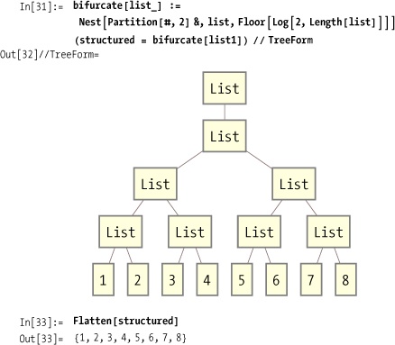
Inner[f,m1,m2,g] is a function that generalizes Dot by allowing a function f to take the place of multiplication and g to take the place of addition. Here are some examples.

You are performing very mathematically intense computations on large vectors, matrices, or higher-order tensors and want the most efficient representation in terms of speed and space.

Make sure your lists are packed arrays by not mixing numerical types. This means arrays of integers should work exclusively in integers or exclusively in machine precision floating point. Use of uniform types is necessary but not sufficient for getting packed arrays. Mathematica tries to automatically use packed arrays when generating large lists of numbers, but sometimes subtle coding differences prevent it from packing the result.

Here are two very similar pieces of code, but the first generates an unpacked representation and the second generates a packed one.

In[66]:=  array1 = N[Table[i * Pi, {i, 0, 500 000}]];
          Developer'PackedArrayQ[array1]
Out[67]=  False

In[68]:=  array2 = Table[i * Pi, {i, 0.0, 500 000.0}];
          Developer'PackedArray'[array2]
Out[69]=  True

The difference is that the first Table generates a table in symbolic form and then converts it to real numbers with N. So, although the final array meets the uniform criteria, N will not pack it. In the second version, I force Table to create a list of real numbers right off the bat by using real bounds for the index i. This makes N unnecessary and causes Table to return a packed result.

To get some insight into the superiority of packed arrays, we can ask Mathematica to tell us the size of each array from the solution.

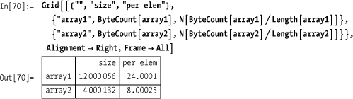
As you can see, the space saved is considerable. Essentially, packed is giving you the equivalent of a C or Fortran array. Space savings is not the only reason to work with packed arrays. Many operations are considerably faster as well. Here you see that multiplication of packed arrays is an order of magnitude faster than unpacked!

In[71]:= Mean@Table[Timing[array1*array2][[1]], {100}]
Out[71]= 0.0909364

In[72]:= Mean@Table[Timing[array2*array2][[1]], {100}]
Out[72]= 0.00625822

When you can get an order of magnitude improvement, it is a good idea to take it, because life is short!

The Developer` package has a function to pack an unpacked array, although it is preferable to alter your coding style as we’ve discussed here to get packed arrays.

In[73]:=  array1 = Developer`ToPackedArray[array1];
          Developer`PackedArrayQ[array1]
Out[74]=  True

Note

If you have a very large packed array and assign a value to one of the elements that differ from the packed type, this assignment will be expensive relative to a normal assignment. Mathematica will be forced to copy the entire array into unpacked form before the assignment can be made.

The Developer` package also has a function Developer`FromPackedArray for converting a packed form back to the normal representation. Evaluating ?"Developer`*" allows you to peruse all the functions in this package, but many are undocumented.

You need to sort a list based on standard ordering (Less) or a custom-ordering relation. One common reason for sorting is to enable binary search.

Use Sort or SortBy, depending on how the ordering relation is specified. By default, Sort uses less than (<) to order elements.

In[76]:=  list = RandomInteger[{-100, 100}, 10];

In[77]:=  Sort[list]
Out[77]=  {-73, -50, -45, -43, -20, 2, 42, 50, 66, 84}

In[78]:=  Sort [list, Greater]
Out[78]=  {84, 66, 50, 42, 2, -20, -43, -45, -50, -73}

SortBy does not use an ordering relation, but rather uses a function whose output is passed to Less.

In[79]:=  SortBy[list, Abs]
Out[79]=  {2, -20, 42, -43, -45, -50, 50, 66, -73, 84}

If you need to sort lists containing objects more complicated than scalars, you will need to be comfortable with expressing the order relation function. Here are some examples.

In[80]:=  data = {
             {"21 Mar 2007 14:34:30", 10.1, 12.7, 13.3},
             {"21 Jun 2005 10:19:30", 10.3, 11.7, 11.7},
             {"21 Aug 2006 15:34:01", 11.7, 16.8, 8.6},
             {"21 Aug 2006 09:34:00", 11.9, 16.5, 8.6}
            };
          (*Sort the data by the time entry,
          which must be converted to an absolute time to be properly ordered.*)
          Sort[data,
            Less[AbsoluteTime[{#1[[1]], {"Day", "MonthNameShort", "Year", "Time"}}],
              AbsoluteTime[{#2[[1]],
                {"Day", "MonthNameShort", "Year", "Time"}}]] &] // TableForm
Out[81]//TableForm=
             21 Jun 2005 10:19:30 10.3 11.7 11.7
             21 Aug 2006 09:34:00 11.9 16.5 8.6
             21 Aug 2006 15:34:01 11.7 16.8 8.6
             21 Mar 2007 14:34:30 10.1 12.7 13.3

For practical sorting, you will never need to look beyond Sort, because it is both fast and flexible. However, if you are interested in sorting from an algorithmic perspective, Mathematica also has a package called Combinatorica`, which contains some sorting routines that use specific algorithms (SelectionSort, HeapSort).

In[82]:=  Needs["Combinatorica`"]

In[83]:=  SelectionSort[list, Less]
Out[83]=  {-73, -50, -45, -43, -20, 2, 42, 50, 66, 84}

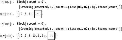
Of course, there is probably no practical reason to use SelectionSort since its asymptotic behavior is O(n^2), whereas Sort uses a O(n log n) algorithm. You can count the number of comparisons each sort makes using a custom comparison function. The framed number is the comparison count.

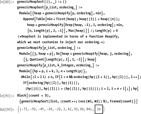
Heap sort is O(n log n), but the Combinatorica` implementation is somewhat crippled because the ordering operation cannot be customized.

In[88]:=  HeapSort[list]
Out[88]=  {-73, -50, -45, -43, -20, 2, 42, 50, 66, 84}

If you are keen to do this experiment with HeapSort, you can easily make a customizable version, since the source code is available.

It is unfortunate that we have to hack HeapSort to give it customizable ordering function. When you develop your own general-purpose functions, it pays to consider facilities that allow you and other users to customize the details while leaving the essential algorithm intact. This is the essence of what is called generic programming. Chapter 2 has several recipes that demonstrate how to create more generic functions.

One application of sorting is performing efficient search. The Combinatorica` package provides the function BinarySearch, which requires a sorted list. BinarySearch returns the index of the first occurrence of a search key, if found. If the key is not found, it returns index + 1/2, indicating that the key belongs between index and index + 1 if it were to be inserted.

3.3 Determining Order Without Sorting discusses how to determine sorted order without rearranging the elements of the list.

A good overview of various sorting algorithms can be found at http://bit.ly/2bRckv .

You need to know how the elements of a list are ordered without actually sorting them. This may be because it is too expensive to keep multiple copies of the data in various orderings.

Use Ordering to get a list of offsets to the elements in the order they would appear if sorted.

In[101]:=  unsorted = Randomlnteger[{90, 99}, 10]
Out[101]=  {98, 90, 91, 98, 98, 91, 99, 99, 97, 96}

In[102]:=  Ordering[unsorted]
Out[102]=  {2, 3, 6, 10, 9, 1, 4, 5, 7, 8}

Ordering has two variations. The first takes an integer that limits how many positions are returned. If you specify n, then the first n are returned; if you specify -n, the last n are returned. This option makes Ordering more useful than Sort when you don’t need the entire list sorted.

In[103]:=  Ordering[unsorted, 3]
Out[103]=  {2, 3, 6}

In[104]:=  Ordering[unsorted, -3]
Out[104]=  {5, 7, 8}

The second variation takes both an integer and an ordering relation.

In[105]:=  ordering[unsorted, Length[unsorted], Greater]
Out[105]=  (8, 7, 5, 4, 1, 9, 10, 6, 3, 2)

Given an ordering, it is easy to create a sorted version of the list.

In[106]:=  unsorted [[Ordering[unsorted]]]
Out[106]=  {90, 91, 91, 96, 97, 98, 98, 98, 99, 99}

Unfortunately, Ordering does as many comparisons as a full sort even if you only want the first few orderings.

A heap would be superior in such an application, but rolling your version of Ordering is unlikely to yield superior results due to optimizations that go beyond minimizing comparisons. After all, it takes Ordering less than a second to do its work on a million integers on my relatively low-powered laptop.

In[109]:=  Timing [Ordering [Randomlnteger [{l, 999 999}, 1000 000], 2]]
Out[109]=  {0.255152, (314075, 337 366))

3.2 Sorting Lists discusses sorting.

OrderedQ tests if a list is ordered, and Order compares two expressions, returning –1 (Less), 0 (Equal), or 1 (Greater).

You want to extract the diagonal, subdiagonal, superdiagonal, or antidiagonal of a matrix.

In versions prior to Mathematica 6, use Tr with List as the combining function (the default combining function of Tr is Plus).

Mathematica 6 introduced the function Diagonal, which makes this recipe trivial.

In[112]:=  Diagonal[matrix]
Out[112]=  {1, 5, 9}

You can extract the antidiagonal using either of the following expressions:

In[113]:=  Diagonal[Map[Reverse, matrix]]
Out[113]=  {3, 5, 7}

In[114]:=  Tr[Map[Reverse, matrix], List]
Out[114]=  {3, 5, 7}

The Diagonal function is more versatile than Tr in that it allows you to select off the main diagonal by proving an index.

In[115]:=  Diagonal[matrix, 1]
Out[115]=  {2,6}

In[116]:=  Diagonal[matrix, -1]
Out[116]=  {4,8}

Although the solutions implementation of antidiagonal is simple, it is not the most efficient: it reverses every row of the input matrix. An iterative solution using Table is simple and fast.

In[117]:=  AntiDiagonal[matrix_] := Module[{len = Length [matrix]},
             Table [matrix [[i, len - i + 1]], {i, 1,len}]]

In[118]:=  bigMatrix = Table[i*j, {i, 0, 5500}, {j, 0, 5500}];

In[119]:=  Timing[AntiDiagonal[bigMatrix]] [[1]]
Out[119]=  0.001839

In[120]:=  Timing [Diagonal[Map[Reverse, bigMatrix]]] [[1]]
Out[120]=  0.230145

It is always good to test a new version of an algorithm against one you already know works.

In[121]:=  AntiDiagonal[bigMatrix] == Diagonal [Map [Reverse, bigMatrix]]
Out[121]=  True

You want to construct matrices of a specific structure (e.g., diagonal, identity, tridiagonal).

Mathematica has built-in matrix constructions for the most common kinds of matrices.

Although identity and diagonal matrices are quite common, there are other kinds of matrices that arise frequently in practical problems. For example, problems involving coupled systems often give rise to tridiagonal matrices. SparseArray and Band are perfect for this job. These are discussed in 3.8 Using Sparse Arrays to Conserve Memory. Here, the use of Normal to convert sparse form to list form is not essential because sparse arrays will play nicely with regular ones.

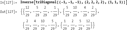
Tridiagonal matrices are always invertible.

There are also functions to transform a given matrix to another. Mathematica 7 introduced LowerTriangularize and UpperTriangularize to create triangular matrices from a given matrix.

These functions take an optional second parameter k, where positive k refers to subdiagonals above the main diagonal and negative k refers to subdiagonals below the main diagonal. This points to another way to arrive at a tridiagonal matrix from a given or synthesized matrix.

Certain important transformation matrices are accommodated by ScalingMatrix, RotationMatrix, and ReflectionMatrix. See 2.11 Computing Through Repeated Function Application for a usage example.

You want to construct a matrix that will permute or shift the rows or columns of an input matrix.

A permutation matrix is a permutation of the identity matrix. It is used to permute either the rows or columns of another matrix.

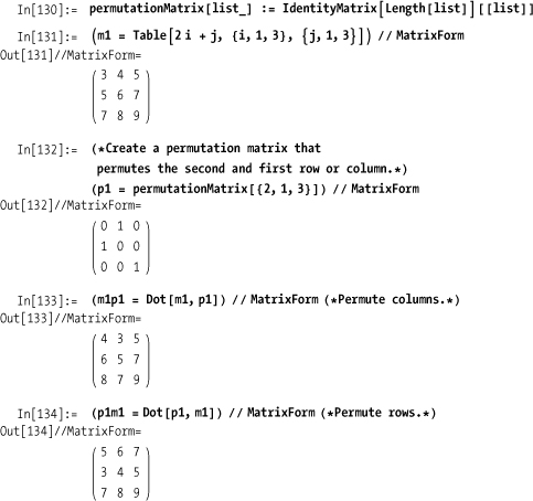
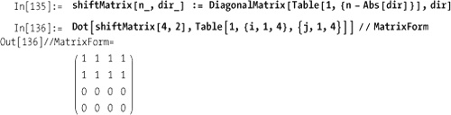
Whereas a permutation matrix permutes rows or columns, a shift matrix shifts rows or columns, replacing the empty elements with zeros. A shift matrix is simply a matrix with Is on the superdiagonal or subdiagonal and 0s everywhere else. This can easily be constructed using the DiagonalMatrix function.

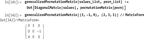
A generalized permutation matrix has the same zero entries as the corresponding permutation matrix, but the nonzero entries can have values other than 1.

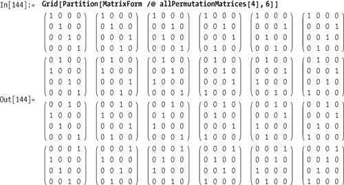
You can easily enumerate all n! permutation matrices of size n.

In[143]:=  allPermutationMatrices[n_] :=
            permutationMatrix[#] & /@ Permutations[Range[n]]

It is also easy to detect if a matrix is a row permutation of another matrix: simply remove each row from ml that matches m2 and see if you are left with no rows. Of course, you must also check that the matrices are the same size. A check for column permutation is just a check for row permutations on the transpose of each matrix.

In[145]:=  isRowPermutation[m1_, m2_] :=
            Length[m1] == Length[m2] && Fold[DeleteCases[#1, #2] &, m1, m2] {}
           isMatrixPermutation[m1_, m2_] := isRowPermutation[ml, m2] ||
             isRowPermutation[Transpose[ml], Transpose[m2]]

You can verify this on some test cases.

In[147]:=  (*Obviously a matrix is a permutation of itself.*)
           isMatrixPermutation[m1, m1]
Out[147]=  True

In[148]:=  (*Test a row permutation.*)
           isMatrixPermutation[m1, p1m1]
Out[148]=  True

In[149]:=  (*Test a column permutation.*)
           isMatrixPermutation[m1, m1p1]
Out[149]=  True

In[150]:=  (*A matrix and its tranpose are not permutations unless symmetric.*)
           isMatrixPermutation [m1, Transpose [m1]]
Out[150]=  False

You may be thinking that matrix permutations via linear algebra will only apply to matrices of numbers, but recall that Mathematica is a symbolic language and, thus, not limited to numerical manipulation. Here we do a Dot product on a matrix of graphics!

This chess demo lacks some aesthetics (the squares move along with the rooks), but it does illustrate the generality of the permutation matrix.

You want to add, remove, or modify entire rows or columns of a matrix in place.

Many operations on lists (including higher-order lists such as matrices) do not modify the input list but rather produce a new list with the change. For example, Append[myList,10] returns a list with 10 appended but leaves myList untouched. Sometimes you want to modify the actual value of the list associated with a symbol.

You may also want to add elements, rows, and columns.

Destructive operations should generally be avoided because they can lead to annoying bugs. For one thing, they make code sensitive to evaluation order. This type of code is harder to change. Further, you need to keep in mind that these operations are being performed on symbols rather than lists. What does this mean? Let’s inspect the attributes of AppendTo to gain a bit of insight.

In[168]:=  Attributes [AppendTo]
Out[168]=  {HoldFirst, Protected}

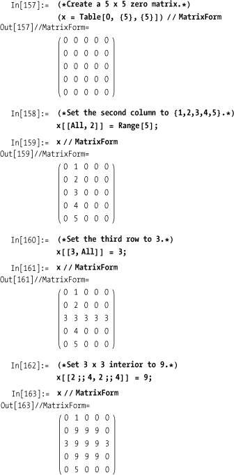
The relevant attribute here is HoldFirst. This means that the expression passed as the first argument is passed in unevaluated form. This has implications when you want to write your own functions that destructively change the value of a symbol. Consider trying to implement your own AppendTo.

First notice that this generated an error message and that x did not change. This occurred because x was evaluated before the call, and you ended up evaluating AppendTo[ List[], 10], which is illegal. You can remedy this by using HoldFirst.

In[174]:=  SetAttributes[myAppendTo, {HoldFirst}]

In[175]:=  myAppendTo[x,10]
Out[175]=  {10}

In[176]:=  x
Out[176]=  {10}

Now it works. As a general rule, you need to use attributes HoldFirst, HoldRest, or HoldAll, as appropriate, to pass expressions in unevaluated form to your own functions. This is covered in 2.0 Introduction and in 2.2 Holding Arbitrary Arguments.

You need to work with very large arrays or matrices but most of the entries are duplicates (typically 0).

Mathematica has direct support for sparse arrays and higher-order tensors using the SparseArray function. The sparse array is built from a rule-based specification that maps positions to values.

You can also specify the positions and values in separate lists. Here is a sparse vector using this technique.

You can also convert a standard matrix to a sparse one.

In[179]:=  dense = DiagonalMatrix[Range[1000]];

In[180]:=  sparse = SparseArray[dense]
Out[180]=  SparseArray[<1000>, {1000, 1000}]

As you can see, the memory savings is considerable.

In[181]:=  ByteCount[dense] - ByteCount[sparse]
Out[181]=  3987416

In[182]:=  ClearAll[dense]

Very large but sparsely populated matrices arise often in applications of linear algebra. Mathematica provides excellent support for sparse arrays because most operations that are available for list-based matrices (or tensors in general) are available for sparse array objects.

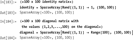
Mathematica does not have sparse equivalents of the convenience functions IdentityMatrix and DiagonalMatrix, but they are easy to synthesize using Band, which specifies either the starting position of a diagonal entry or a range of positions for a diagonal.

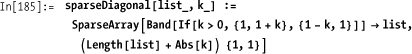
A general sparse diagonal function looks like this.

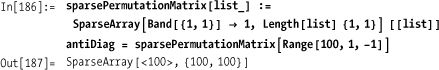
You can also produce sparse versions of the permutation matrices from 3.6 Constructing Permutation and Shift Matrices.

3.5 Constructing Matrices of Specific Structure showed how to use SparseArray and Band to create tridiagonal matrices.

You need to extract, delete, modify, or transform content deep inside a nested list.

A level specification (or levelspec) is the key for surgically manipulating lists that contain many levels. Most of Mathematica’s functions that deal with lists have variations that take levelspecs. Position is one such function. Consider a list of integers that has values nested up to eight levels.

If you use Position to search for 1, you get a list of all positions that have the value 1.You can verify this using Extract.

In[191]:=  Position [deep, 1]
Out[191]=  {{1}, {2, 5, 1}, {2, 5, 3}, {2, 6, 1}, {2, 6, 2, 1, 1, 1, 1},
            {2, 6, 2, 1, 1, 2}, {2, 6, 2, 1, 2, 1}, {2, 6, 2, 2}, {2, 7}, {2, 8}, {2, 9}}

In[192]:=  Extract [deep, Position [deep,1]]
Out[192]=  {l,l,l, 1, 1, 1, 1, 1, 1, 1, 1}

Suppose you do not want the Is at every level. This is where levelspecs come in handy.

Use a single positive integer n to search at all levels up to and including n.

In[193]:=  (*Only search up to level two.*)
           Position [deep, 1, 2]
Out[193]=  {{1}, {2, 7}, {2, 8}, {2, 9}}

Enclosing the level {n} in a list restricts search to that level.

In[194]:=  (*Only search at level two.*)
           Position [deep, 1, {2}]
Out[194]=  {{2, 7}, {2, 8}, {2, 9))

The list notation {n,m} restricts search to levels n through m, inclusively.

In[195]:=  (*Search at levels three through five.*)
           Position [deep, 1, {3, 5}]
Out[195]=  {{2, 5, 1}, {2, 5, 3}, {2, 6, 1}, {2, 6, 2, 2}}

Negative level specification of the form -n looks for objects that themselves have depth n.

In[196]:=  Position [deep, 1, -1]
Out[196]=  {{1}, {2, 5, 1}, {2, 5, 3}, {2, 6, 1}, {2, 6, 2, 1, 1, 1, 1},
            {2, 6, 2, 1, 1, 2}, {2, 6, 2, 1, 2, 1}, {2, 6, 2, 2}, {2, 7}, {2, 8}, {2, 9}}

In[197]:=  (*See the discussion for why this is empty and must be empty.*)
           Position [deep, 1, -2]
Out[197]=  {}

We used Position to get a feel for level specifications because it is easy to judge, based on the length of each position sublist, the depth of each item found. However, you may be surprised that the last example was empty. It is easy to mistakenly think that negative level specification means searching from the bottom of the tree up because this seems analogous to the way negative indices work in functions like Part. This is not the case. A negative level specification means only looking for items with specified depth after dropping the minus sign. Any scalar (like 1) has depth 1, including complex numbers.

In[198]:=  {Depth[1], Depth[3.7], Depth["foo"], Depth[1 + 7 I]}
Out[198]=  {1, 1, 1, 1}

From this, it follows that a scalar will never be found by using a negative depth value less than -1.

Another important function for illustrating the use of level specifications is Level. Its function is to retrieve all objects at the specified level(s).

In[199]:=  Level [deep, {2}]
Out[199]=  {2, 3, 4, 5, {1, 6, 1, 7}, {1, {{{{1, 8}, 1}, {1}}, 1}}, 1, 1, 1, 9, 10, 11}

Objects at level {2} may have a variety of depths.

In[200]:=  Depth /@ Level [deep, {2}]
Out[200]=  {1, 1, 1, 1, 2, 6, 1, 1, 1, 1, 1, l}

Objects at level {-2} will only have a single depth by definition.

In[201]:=  Level [deep, {-2}]
Out[201]=  {{1, 6, 1, 7}, {1, 8}, {1}}

In[202]:=  Depth /@ Level [deep, {-2}]
Out[202]=  {2, 2, 2}

A picture helps reinforce this. Note that each tree has two levels.

Note the difference between {-2}, meaning exactly depth 2, and -2, meaning depth 2 or more.

In[204]:=  Depth /@ Level [deep, -2]
Out[204]=  {2, 2, 3, 2, 4,5,6, 7}

Once you have mastered level specifications, the functions Apply, Cases, Delete, DeleteCases, Extract, FreeQ, Level, Map, Maplndexed, MemberQ, Position, Replace, and Scan take on more power and precision because they each have versions that use levelspecs.

Here are some examples in which we extract, delete, and modify the contents of a deeply nested expression. This time we use an algebraic expression.

Chapter 2, has recipes that deal with the specifics of Apply, Map, Maplndexed, and Scan.

Chapter 4, has recipes that deal with the specifics of Cases, DeleteCases, FreeQ, MemberQ, and Replace

You want to manipulate a vector of bits in a space-efficient fashion. You also want to give these vectors a concise default display format.

You can use Mathematica’s ability to represent arbitrarily large integers as a means of implementing bit vectors. Using Mathematica’s UpValue convention (see Chapter 2, DownValues and UpValues) you can make bit vectors adopt the familiar interface used by lists. When you create custom data structures like this, you can give them an output format that hides the details of their internal representation.

In[215]:=  (*Make a bit vector from a list of bit value.*)
           makeBitVector[bits_List] :=
            bitvec[FromDigits[Reverse[bits], 2], Length[bits]]
           (*Make a bit vector of a specified
            length. Values are initialized to 0.*)
           makeBitVector[1_: 32] := bitvec[0, 1]
           (*Set bit at index to 0 or 1.*)
           setBit [bitvec[n_, 1_], index_Integer, 1] :=
            Module[ {n2 = BitSet[n, index -1]}, bitvec[n2, Max[1, BitLength[n2]]]]
           setBit [bitvec[n_, 1_], index_Integer, o] :=
            bitvec[BitClear [n, index - 1], 1]
           SetAttributes[setBitOf, HoldFirst]
           setBitOf [name_symbol, index_Integer, bit_ /; bit === 0 || bit === 1] :=
            name = setBit [name, index, bit]
           (*Get the first bit value.*)
           bitvec /: First [bitvec[n_, _]] := BitGet[n, 0]
           (*Get the rest of the bits after the first as a new bit vector.*)
           bitvec /: Rest [bitvec [n_, 1_]] := bitvec [Floor [n / 2],1 - 1]
           (*Get bit at index.*)
           bitvec /: Part [bitvec[n_, _], index_Integer] := BitGet [n, index - 1]
           (*Get the length of the bit vector.*)
           bitvec /: Length [bitvec [n_, 1_]] := 1
            bitvec /: BitLength [bitvec [n_, 1_]] := 1
           (*Perform bitwise AND of two vectors.*)
           bitvec /: BitOr[bitvec[ n1_, 11_], bitvec[ n2 _, 12_]]:=
            bitvec [BitOr[n1, n2], Max [11,12]]
           (*Perform bitwise OR of two vectors.*)
           bitvec /: BitOr [bitvec [n1_, 11_], bitvec [n2_, 12_]]:=
            bitvec[BitAnd [n1, n2], Max [11, 12] ]
           (*Return the complement (NOT) of a bit vector.*)
           bitvec /: BitNot [bitvec[ n _, 1_]] :=
            bitvec[BitAnd [BitNot [n], 2 ^ 1 - 1], 1]
           (*Create a format to print bit vectors in an abbreviated fashion.*)
           Format [bitvec[ n _, 1_]] :=
            "bitvec"["<"<> Tostring[BitGet[n,o]] <> " ••• " <>
              ToString [BitGet [n, 1 - 1]] <> ">", 1]

Here are some examples of usage.

In[229]:=  bv = makeBitVector[{1, 0, 0, 0, 1}]
Out[229]=  bitvec[<1...1>, 5]

In[230]:=  bv[[2]]
Out[230]=  0

In[231]:=  bv = setBit[bv, 2, 1]
Out[231]=  bitvec[<1...1>, 5]

In[232]:=  bv[[2]]
Out[232]=  1

In[233]:=  bv = setBit[bv, 500, 1]
Out[233]=  bitvec[ <1...1>, 500]

In[234]:=  bv2 = Rest[bv]
Out[234]=  bitvec[<1...1>, 499]

In[235]:=  bv3 = BitNot[makeBitVector[{1, 0, 0, 0, 1}]]
Out[235]=  bitvec[<0...0>, 5]

In[236]:=  bv3 [[1]]
Out[236]=  0

Even if you have no immediate application for bit vectors, this recipe provides a lesson in how you can create new types of objects and integrate them into Mathematica using familiar native functions.

See tutorial/DefiningOutputFormats in the Mathematica documentation for more details on Format.

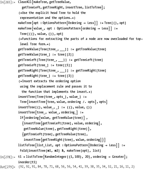
You want to model tree data structures in Mathematica and operate on them with standard tree-based algorithms.

The simplest tree is the binary tree, and the simplest model of a binary tree in Mathematica is a list consisting of the left branch, node value, and right branch.

In[238]:=  (*MakeTree constructs either an empty
            tree or a tree with only a root element.*)
           makeTree[] := {}
           makeTree[value_] := {{}, value, {}}
           (*Functions for extracting the parts of a node*)
           getTreeValue[tree_] := tree [[2]]
           getTreeLeft[tree_] := tree[[l]]
           getTreeRight[tree_] := tree[[3]]
           (*We insert elements into a tree using < ordering relation.*)
           insertTree[{}, value _] := {{}, value, {}}
           insertTree[tree_, value_] := If[value < getTreeValue[tree],
             {insertTree [getTreeLeft[tree], value],
              getTreeValue[tree], getTreeRight[tree]},
             {getTreeLeft[tree], getTreeValue[tree],
              insertTree[getTreeRight[tree], value]}]
           (*Given the above primitives, it is easy to define
            some common algorithms.*)
           listToTree[list_List] := Fold[insertTree[#1, #2] &, makeTree[], list]
           (*A preorder traversal is also known as depth-first.*)
           preorder[tree_] := Reap[preorder2[tree]] [[2, 1]]
           preorder2[{}] := {}
           preorder2[tree_] := Module[{}, Sow[getTreeValue[tree]];
                                     preorder2[getTreeLeft[tree]];
                                 preorder2[getTreeRight[tree]]]
        postorder [tree_] := Reap [postorder2 [tree]][[2, 1]]
        postorder2[{}] := {}
        postorder2[tree_] := Module[{},
          postorder2[getTreeLeft[tree]];
          postorder2[getTreeRight[tree]];
              Sow[getTreeValue[tree]];
        (*An inorder traversal returns the values in sorted order.*)
        inorder[tree_] := Reap[inorder2[tree]][[2, 1]]
        inorder2[{}] := {}
        inorder2[tree_] := Module[{},
          inorder2[getTreeLeft[tree]];
          Sow[getTreeValue[tree]];
          inorder2[getTreeRight[tree]]]
         (*A level order traversal is also known as breadth first.*)
         level order[tree_] := Reap[levelorder2[{tree}]][[2, 1]]
         (*Breadth first is commonly implemented in terms of
          a queue that keeps track of unprocessed levels. I model
          the queue as a list.*)
         levelorder2[{}] := {} (*Stop on empty queue.*)
         levelorder2[{{}}] := {} (*Stop on queue with empty tree.*)
         levelorder2[queue_] := Module[{front = First [queue],
            queue2 = Rest[queue], (*Pop front of queue.*),
            left, right},
           Sow[getTreeValue[front]]; (*Visit node. *)
           left = getTreeLeft[front];
           right = getTreeRight[front];
           queue2 = If[Length[left] == 0, queue2, Append[queue2, left]];
           (*Append left if not empty.*)
           queue2 = If[Length[right] == 0, queue2, Append[queue2, right]];
           (*Append right if not empty.*)
           levelorder2[queue2]]

In[259]:=  nodes = RandomInteger[{1, 100}, 18]
Out[259]=  {62, 97, 36, 82, 76, 84, 58, 32, 79, 16, 89, 15, 45, 72, 90, 32, 12, 9}

The tree implementation in the solution is a bit simplistic, but it is intended to illustrate basic concepts. One way to generalize the implementation is to allow a different ordering function. It makes sense to keep the ordering with each instance of the tree. For this, it is best to use Mathematica options, which are a standard convention for optional values. You need to redefine the functions for creating trees and accessing their parts, but once you do that, the existing algorithm implementations will still work.

Another enhancement is to generalize the so-called visit function of the traversal algorithms.

In[280]:=  ClearAll[inorder, inorder2];
           inorder[tree_, visit_ : Sow] := Flatten[Reap[inorder2[tree, visit]]]
           inorder2[ {},_] := {}
           inorder2[tree_, visit_] := Module [{},
            inorder2[getTreeLeft[tree], visit];
            visit[getTreeValue[tree]];
            inorder2[getTreeRight[tree], visit]]

This allows the caller the option of not receiving all the nodes. For example, rather than Sow, you can pass in a function that writes the values to a file or a filter as we do here.

In[284]:=  inorder [t1, If[OddQ [#], SOW [#], #] &]
Out[284]=  {91, 71, 41, 39, 35, 21, 11}

More information on trees and tree traversal can be found in any computer science data structures book or at http://bit.ly/7xP6jQ.

You need better-than-linear associative lookup and storage to increase performance of a program. You also need the elements to remain ordered.

A red-black tree is a popular balanced tree algorithm used as the foundation for associative data structures. To implement a red-black tree in Mathematica, you create a representation of the tree and functions for creating, reading, updating, and deleting (CRUD). This implementation will use a head rbTree containing a tree and an ordering relation. The tree is modeled as either an empty list or a quadruple consisting of a color (red or black), a left subtree, an element, and a right subtree. By default, we use the function Less as the ordering relation. Storing the ordering relation as part of the tree allows for trees of varying element content.

In[285]:=  (*Make an empty tree with default ordering.*)
           makeRBTree[] := rbTree[ {}, Less]
           (*Make an empty tree with a custom ordering.*)
           makeRBTree[ordering_] := rbTree[{}, ordering]
           (*Make a tree with given root and ordering.*)
           makeRBTree[{color_, left_, elem_, right_), ordering_] :=
            rbTree[{ color, left, elem, right}, ordering]

Before we can do much with these trees, we need a method for inserting new elements while keeping the tree well ordered and balanced. For this, we create a toplevel insert function implemented in terms of several low-level functions that maintain all the constraints necessary for a red-black tree.

In[288]:=  insertRBTree[rbTree[struct_, ordering_], elem_] :=
            makeRBTree[makeBlack[insertRBTree2[struct, elem, ordering]], ordering]

In[289]:=  (*This implementation method does ordered
            insertion and balancing of the tree representation.
             Note: empty subtrees {} are considered implicitly black.*)
           insertRBTree2[{}, elem_, _] := {red, {}, elem, {}}
           insertRBTree2[{color_, left_, elem2_, right_}, elem1_, ordering_] :=
             Which[ordering[elem1, elem2],
             balance[color, insertRBTree2[left, elem1, ordering], elem2, right],
                   ordering[elem2, elem1],
             balance[color, left, elem2, insertRBTree2[right, elem1, ordering]],
                    True, {color, left, elem2, right}]
In[291]:=  (*This is a helper that turns a node to black.*)
           makeBlack[{color_, left_, elem_, right_}] := {black, left, elem, right}
In[292]:=  (*Balancing is handled by a transformation function that
             matches all red-black constraint violations
             and transforms them into balanced versions.*)
           balance[black, {red, {red, left1_, elem1_, right1_}, elem2_, right2_},
             elem3_, right3_]:=
            {red, {black, left1, elem1, right1}, elem2, {black, right2, elem3, right3}}
           balance[black, {red, left1_, elem1_, {red, left2_, elem2_, right1_}},
             elem3_, right2_] :=
            {red, {black, left1, elem1, left2}, elem2, 
             {black, right1, elem3, right2}}
           balance[black, left1_, elem1_,
              {red, {red, left2_, elem2_, right1_}, elem3_, right2_}]:=
             {red, {black, left1, elem1, left2}, elem2,
              {black, right1, elem3, right2}}
           balance[black, left1_, elem1_,
              {red, left2_, elem2_, {red, left3_, elem3_, right1_}}] :=
             {red, {black, left1, elem1, left2}, elem2, {black, left3, elem3, right1}}
           balance[color_, left1_, elem1_, right1_] :=
             {color, left1, elem1, right1}

List-to-tree and tree-to-list conversions are very convenient operations for interfacing with the rest of Mathematica.

There are several ways to approach a problem like this. One reasonable answer is to implement associative lookup outside of Mathematica using a language like C++ and then use MathLink to access this functionality. Here we will take the approach of implementing a red-black tree directly in Mathematica.

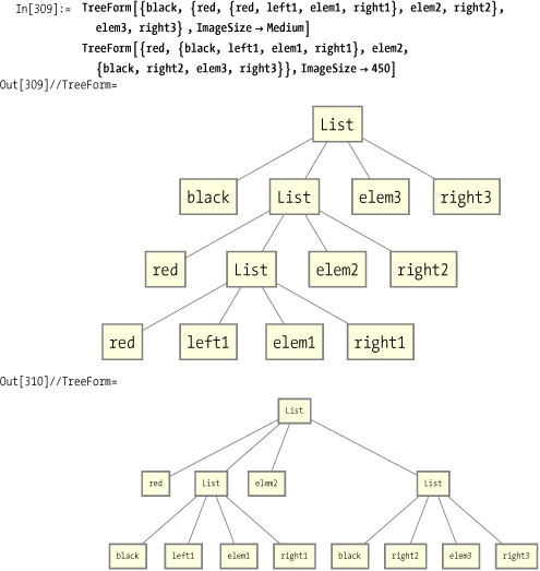
A red-black tree implemented in C may typically be hundreds of lines of code, yet we achieve an implementation in Mathematica with less than a hundred, including comments. How is this possible? The main idea is to exploit pattern matching as much as possible. Note particularly the function balance. This function directly implements the most tricky part of a red-black-tree implementation in a traditionally procedural language by stating the balancing rules in a form that is very close to the way the algorithm requirements might specify them. Let’s take one of the versions as an example.

balance[black, {red, {red, left1_, elem1_, right1_}, elem2_, right2_}, elem3
_, right3_] :=
 {red, {black, left1, elem1, right1}, elem2, {black, right2, elem3, right3}}

The above says: "If you find a black node (elem3) with a red left child (elem2) that also has a red left child (elem1), then convert to a red node with two black children (elem1 and elem3, in that order). This is a case where the code speaks more clearly and precisely than any English translation. With a slight bit of editing, the code itself translates into a graphical view of before and after. I can‘t think of another general programming language where you can code and visualize an algorithm with so little added effort!

A solution to associative lookup that is more in the spirit of Mathematica can be found in 3.13 Exploiting Mathematica’s Built-In Associative Lookup.

This recipe was inspired by the book Purely Functional Data Structures by Chris Okasaki (Cambridge University Press), in which Haskell is used to demonstrate that data structures can be written under the constraints of a pure functional programming language.

Wikipedia provides a good basic explanation of and references to more sources for red-black trees ( http://bit.ly/3WEqrT ).

You want to create a dictionary to associate keys with values, but you want Mathematica to do most of the work.

Harness the same mechanism Mathematica uses to locate the downvalues of a symbol to create the dictionary.

Here I outline the basic idea for the solution and defer the actual implementation to the discussion. The idea is simply to exploit something that Mathematica must already do well: look up a symbol’s downvalues. It must do this well because it is central to Mathematica programming. Imagine you want to create a table of values associating some U.S. zip codes with towns. A reasonable way to proceed is as follows:

In[311]:=  zipcode[11771] = {"Oyster Bay", "Upper Brookville",
               "East Norwhich", "Cove Neck", "Centere Island"};
           zipcode[11772] = {"Patchogue", "North Patchogue", "East Patchogue"};
           (*And so on...*)
           zipcode [11779] = {"Ronkonkoma", "Lake Ronkonkoma"};

Now, when your program needs to do a lookup, it can simply call the "function" zipcode.

This is so obvious that few regular Mathematica programmers would even think twice about doing this. However, this use case is static. Most associative data structures are dynamic. This is not a problem because you can also remove downvalues.

In[315]:=  zipcode[11779] =.

Now there is no longer an association to 11779. Mathematica indicates this by returning the expression in unevaluated form.

In[316]:=  zipcode[11779]
Out[316]=  zipcode[11779]

But this is still not enough. An associated data structure should also tell you all the keys and all the values it knows. Again, Mathematica comes through.

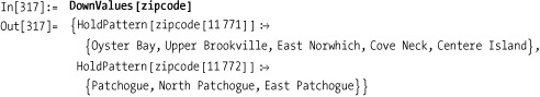
So all the building blocks are present in the core of Mathematica to create a dynamic dictionary-like data structure. All that is needed is the creation of some code to neatly tie these pieces together into a general utility.

The first function we need is a way to construct a dictionary. In the solution, we use a symbol that makes sense for the problem at hand, but in a generic implementation what symbol is used is not significant so long as it is unique. Luckily, Mathematica has the function Unique to deliver the goods. We initialize the dictionary by creating a downvalue that maps any value to the empty list. The symbol is wrapped up in the head Dictionary and returned to the caller.

In[318]:=  makeDictionary[] :=
                Module [{name},
                     name = Unique ["dict"];
                     Evaluate [name] [k_] := {};
                     Dictionary [name]
                ]

You will also want a way to get rid of dictionaries and all their content. Remove does the trick.

In[319]:=  destroyDictionary[Dictionary[name_,_]] :=
            If[ValueQ[name[_] ], Remove[name]; True, False]

Although we said that there is no need to know the symbol used internally, there is no harm in providing a function to retrieve it. Further, our implementation will use this function so that it is easier to change the internal representation in the future.

In[320]:=  dictName[Dictionary[name_,_]] := name

The most important function, dictStore, allows the association of a value with a key. We assume, as in the solution, that more than one value may be needed for a given key, so we store values in a list and prepend new values as they are added.

In[321]:=  dictstore[dict_Dictionary, key_, value_] :=
            Module[{d = dictName[dict]}, d[key] = Prepend[d[key],value]]

The function dictReplaee is like dictStore, except it guarantees value is unique. That is, there are no duplicates of value, although there might be other values for the key.

In[322]:=  dictReplace [dict_Dictionary, key _, value] :=
            Module[{d = dictName[dict]}, d[key] = d[key]∪(value}]

In contrast, the function dictRemove ensures that there are no instances of value associated with the key (although, again, there might be other values for the key).

In[323]:=  dictRemove[dict_Dictionary, key-, value] :=
            Module[{d =dictName [dict]}, d[key] = Complement [d [key], {value}]]

If you want all values removed, then use dict Clear.

In[324]:=  dictClear[Dictionary[name_, _]] :=
            If[ValueQ[name[_]], Clear[name]; Evaluate[name][k_] := {}; True, False]

Maintaining the dictionary is all well and good, but you also need to be able to retrieve values. The function dictLookup is the easiest to implement because it gets Mathematica to do all the work by simply asking for the downvalue in the usual way.

In[325]:=  dictLookup[Dictionary[name_, _], key] := name[key]

Sometimes you might not care what the value is but rather if the key exists at all. Here I use ValueQ, which returns true if the evaluation of an expression returns something different than the expression itself (hence, indicating there is a value). In this implementation, I don‘t care that the value may be the empty list {} because dictHasKeyQ is only intended to tell the caller that the key is present.

In[326]:=  dictHasKeyQ[Dictionary[name_, _], key] := ValueQ [name [key]]

This function tells you that the key is present but has no values.

In[327]:=  dictKeyEmptyQ[Dictionary[name_,_],key]:= name[key] === {}

In some applications, you may want to know the set of all keys; dictKeys provides that. It works by using DownValues, as shown in the solution, but transforms the results to extract only the keys. Most is used to exclude the special downvalue name[k_], which was created within makeDictionary. The use of HoldPattern follows from the format that DownValues uses, as seen in the solution section. Here, Evaluate is used because DownValues has the attribute HoldAll.

Another useful capability is to get a list of all key value pairs; dictKeyValuePairs does that.

Before I exercise this functionality, a few general points need to be made.

You may be curious about the pattern Dictionary[name_, _] since the representation of the dictionary, per makeDictionary, is clearly just Dictionary[name]. As you probably already know (see Chapter 4 if necessary), _ matches a sequence of zero or more expressions. Using this pattern will future proof the functions against changes in the implementation. For example, I may want to enhance Dictionary to take options that control aspects of its behavior (for example, whether duplicate values are allowed for a key or whether a key can have multiple values all together). Keep this in mind when creating your own data structures.

A collection of functions like this really begs to be organized more formally as a Mathematica package. In fact, you can download such a package, with the source code, at this book’s website, http://oreilly.com/catalog/9780596520991/. I cover packages in 18.4 Packaging Your Mathematica Solutions into Libraries for Others to Use.

Here is how I might code the zip codes example from the solution if I needed the full set of create, read, update, and delete capabilities that Dictionary provides.

In[330]:=  zipcodes = makeDictionary[];
           dictStore[zipcodes, 11771,#] & /@ {"Oyster Bay",
              "Upper Brookville", "East Norwhich", "Cove Neck", "Centere Island"};
           dictStore [zipcodes, 11772,#] &/@
              {"Patchogue", "North Patchogue", "East Norwhich"};
           dictStore [zipcodes, 11779,#] &/@ {"Ronkonkoma", "Lake Ronkonkoma"};

In[334]:=  dictLookup[zipcodes, 11771]
Out[334]=  {Centere Island, Cove Neck, East Norwhich, Upper Brookville, Oyster Bay}

In[335]:=  dictLookup[zipcodes, 99999]
Out[335]=  {}

Ask if a key is present.

In[336]:=  dictHasKeyQ[zipcodes, 11779]
Out[336]=  True

Get all the zip codes stored.

In[337]:=  dictKeys[zipcodes]
Out[337]=  {11771, 11772, 11779}

In 3.12 Implementing Ordered Associative Lookup Using a Red-Black Tree quite a bit more coding is required to get a similar level of functionality. This recipe is relatively easy because it leverages one of Mathematica’s strengths. This is an important lesson when working with Mathematica (or any language). Always look for solutions that play to the language’s strengths rather than using hack solutions designed for other programming environments. To be fair, the red-black-tree implementation has features that would be more difficult to support in this recipe. Specifically, we could control the ordering of keys with red-black tree, but here keys are ordered according to Mathematica’s conventions (which are conveniently in line with the expectations one would have for a dictionary).

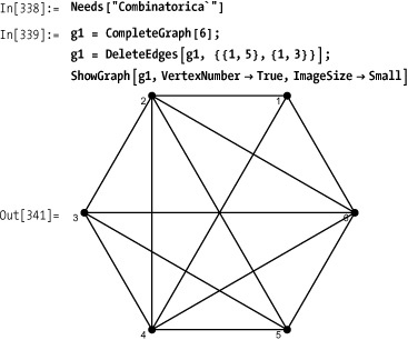
You are solving a problem modeled as a graph and need to create that graph for use with Combinatorica' package’s algorithms.

If your graph is almost complete, construct a complete graph and remove unwanted edges.

If your graph is sparse, construct directly.

Use MakeGraph if your graph can be defined by a predicate.

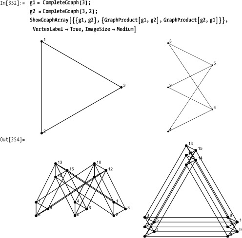
Graphs can also be constructed from combinations of existing graphs by using GraphUnion, GraphIntersection, GraphDifference, GraphProduct, and GraphJoin. In the examples given here, I always use two graphs, but the operations are generalized to multiple graphs.

GraphUnion always creates a disjoint graph resulting from the combination of the graphs in the union.

GraphJoin performs a union and then links up all the vertices from the corresponding graphs.

GraphIntersection works only on graphs with the same number of vertices and produces a graph where the input graphs have edges in common.

GraphDifference creates a graph with all the edges that are in the first graph but not in the second.

GraphProduct creates a graph by injecting copies of the first graph into the second at each vertex of the second and then connecting the vertices of the injected graphs.

Unlike a numerical product, this operation is not commutative, as demonstrated in Out[354] on Discussion.

Another way to construct graphs is from alternate representations, such as adjacency matrices and adjacency lists. Out[355] on Discussion shows a graph constructed from an adjacency matrix obtained from GraphData. Normal is used to convert SparseMatrix, since Combinatorica does not recognize sparse-matrix representations.

Combinatorica also supports directed graphs and graphs with weighted edges. Using SetEdgeWeights alone gives random real weights in the range [0,1]. SetEdgeWeights also accepts Weighting Function and WeightRange options. You can also explicitly specify the weights in a list, which will be assigned to the edges in the same order as returned by the function Edges.

The definitive reference to Combinatorica is Computational Discrete Mathematics: Combinatorics and Graph Theory with Mathematica by Sriram Pemmaraju and Steven Skiena (Cambridge University Press). This reference is essential if you intend to use Combinatorica in a serious way, because the documentation that comes bundled with Mathematica is very sparse.

Mathematica has an alternate graph package called GraphUtilities‘ that represents graphs using lists of rules (e.g., {a → b, a → c, b → c}). There is a conversion function to Combinatorica` graphs. Search for GraphUtilities in the Mathematica documentation.

You want to test a graph for specific properties or find paths through a graph with specific properties or which satisfy specific constraints.

There are many graph theoretic functions in the Combinatorica` package related to shortest paths, network flows, connectivity, planarity testing, topological sorting, and so on. The solutions and following discussion show a sampling of some of the more popular graph algorithms.

Out[363]a shows a graph generated from a complete graph with select edges removed. The graph in Out[363]b is the minimum spanning tree of Out[363]a, and Out[363]c is the shortest path spanning tree.

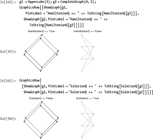
Properties of graphs can be tested using a variety of functions, such as HamiltonianQ (which has a cycle that visits each vertex once), EulerianQ (which has a tour that traverses each edge once), AntisymmetricQ, ReflexiveQ, UndirectedQ, Self LoopsQ, and so on. There are over 40 such predicates in Combinatorica.

A directed graph with no cycles is called a directed acyclic graph (DAG). The transitive closure of a DAG is the supergraph that adds directed edges from ancestors to descendants.

In[367]:=  g = CompleteBinaryTree[7];
           e = Reverse[Edges[g], {2}];
           g = DeleteEdges [MakeDirected [g], e];
           {AcyclicQ[g],TopologicalSort[TransitiveClosure[g]]}
Out[370]=  {True, {1, 2, 3, 4,5,6, 7})

Out[371] shows the tree and its transitive closure. When you display highly connected graphs (like the transitive closure) with vertex labels, it often helps to use opacity or font control to make sure vertex labels are not obscured by the edges.

See Chapter 7 and Chapter 8 in Computational Discrete Mathematics: Combinatorics and Graph Theory with Mathematica by Sriram Pemmaraju and Steven Skiena.