You are solving a problem by incremental refinement of a set of functions. As you proceed to refactor and introduce alternative definitions for symbols, you find that code that was working before mysteriously breaks.

Make judicious use of Clear before every group of functions that are still undergoing development. First, I illustrate what can go wrong if you are sloppy. Suppose you define this function f.

f[x_Integer] := x^2;

Later, you decide that you should be more general about the valid types for argument x and also realize you really meant to compute x^2 +1, so you change the line to this (deleting the previous line from the notebook):

f[x_?NumericQ] := x^2 + 1

Later (possibly after you have forgotten the old version even existed), you try out your code and are surprised by the result.

f[2]
4

To avoid problems like this, you should clear old definitions before defining a function. Then you can redefine f to your heart’s content without worrying that old definitions will interfere.

Clear[f]
f[x_?NumericQ] := x^2 + 1

Developers coming from other programming environments easily fall into the trap caused by the fact that the kernel holds all definitions created during a session unless they are specifically cleared or exactly redefined. This is not the expected behavior of languages that are compiled or interpreted, since in those environments old definitions do not persist. The solution shows one way problems can arise, but there are others. It is just as likely that conflicts can come from other notebooks that are sharing the same kernel instance. Many Mathematica veterans begin their notebooks with an expression to clear every symbol in the global context (a context is similar to what other languages call namespaces).

Clear["Global'*"]

The Global` context is the default context in which new symbols are defined.

You can also clear the command history. This is useful for freeing memory. Consider the following example.

In[192]:= MemoryInUse[]
Out[192]= 132430904

Let’s use a lot of memory.

In[193]:= x = Array[f, {1000, 1000}];
          MemoryInUse[]
Out[194]= 188 470 896

Simply clearing x does not get the memory back because it is cached in the history.

In[196]:=  Clear[x];
           MemoryInUse[]
Out[197]=  188 473 032

However, you can clear the In and Out history by unprotecting, clearing, and repro-tecting In and Out.

In[198]:=  Unprotect[In, Out];
           Clear[In, Out];
           Protect[In, Out];
           MemoryInUse[]
Out[201]=  132 287 208

Problems with name conflicts can also be mitigated by use of packages. See 18.4 Packaging Your Mathematica Solutions into Libraries for Others to Use.

You want to extend or alter the meaning of intrinsic functions that are built in to Mathematica. Perhaps you want to introduce a mathematical object that has its own natural definitions for the standard operations Plus, Times, etc.

The most straightforward way to modify Mathematica operations is to unprotect them, augment their meaning, and protect them again. However, the easiest way is frequently not the best or safest way, so be sure not to skip the "Discussion" section.

It is common in certain applications to consider 0^0 to be defined as 1; however, Mathematica considers this expression to be indeterminate and will issue a warning when it evaluates it (hence, the use of Quiet here).

0^0 // Quiet
Indeterminate

You can change this behavior quite easily.

Unprotect[Power];
Power[0,0] = 1;
Protect[Power];
0^0
1

This new behavior will persist only within the Mathematica kernel session and will be known to all notebooks associated with the notebook’s kernel. See 18.9 Initializing and Cleaning Up Automatically for a way to make such changes automatically active each time you use Mathematica.

The solution shows a reasonable change to the meaning of an intrinsic function. It is reasonable because it is unlikely to change the behavior of Mathematica in a detrimental way since you are simply supplying meaning to an expression that had no meaning. Technically speaking, it is possible that third-party code you are also using depended on Power[0,0] evaluating to indeterminate; however, this possibility is farfetched. This is not the case for other seemingly reasonable changes. For example, you might be irked by the following result:

(-1) ^ (1/3) //N
0.5 + 0.866025 i

Clearly, an equally valid answer is -1. In fact, there are three valid answers. This is a question of which branch Mathematica takes by default.

To remedy this choice, you might decide to take matters into your own hands and force Mathematica to take a different branch whenever it needs to evaluate a rational power of a negative number.

Unprotect[Power];
Power[a_ ?Negative, n_Rational] = Exp[n Log[a] + n 2 Pi I];
Protect[Power];
(-1) ^ (1/3) //N
-1.

This has an unfortunate consequence if you want Solve to work as before!

Quitting the kernel will revert to the old behavior.

Sometimes you want to temporarily change the meaning of a symbol. In that case, use of Unprotect is overkill, and it is better to introduce the new value within a Block. For example, E is the built-in symbol for the base of the natural logarithm, but in this block we use E as hex digit 14.

Block[{A = 10, B = 11, C = 12, D = 13, E = 14, F = 15}, A * 16 + E]
174

This technique is often used to temporarily change special global variables like $RecursionLimit. The following is a recursive implementation of the Ackermann function that would easily overflow the default stack limit of 256. This is for illustration purposes and not a good way to implement Ackermann.

(*Ackermann function*)
Block[{$RecursionLimit = 100000, A},
 A[0, n_] := n + 1; A[m_, 0] := A[m, 0] = A[m - 1,1];
 A[m_, n_] := A[m, n] = A[m-1, A[m, n-1]]; A[4, 1]]
65 533

You are wondering what undocumented functions might be hiding in your current version of Mathematica.

Inspect the Developer` and Experimental` contexts for hidden treasures. Here, //Short is used only to reduce clutter, so remove that before evaluating.

  In[891]:=  Names["Developer`*"] // Short
Out[891]//Short=

             {Developer`BesselSimplify, <<69>>, Developer`$SymbolSystemShadowing }

  In[892]:=  Names["Experimental`*"] // Short
Out[892]//Short=

             {Experimental`AngleRange, <<47>>, Experimental`Wait }

Strictly speaking, the Developer` context is not entirely undocumented, but rather consists of low-level access to underlying algorithms that are typically used in the implementation of higher-level, built-in functions. Here is an example of such a function and its documentation. However, you can see that the documentation is much more sparse than that of a function available in standard System` context.

In contrast, expect to find little information about functions in the Experimental` context.

Even if you manage to figure out how these functions work, there is no guarantee the functions won’t change or be removed in a future version, so use them with caution. Sometimes an experimental function will tell you it has been deprecated and direct you to an alternative.

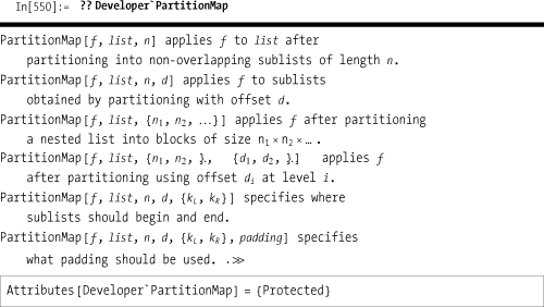
PartitionMap was used in 2.6 Mapping a Function over a Moving Sublist.

You have a nice collection of functions that are of general use within your organization or perhaps as a library that you want to distribute to others.

Mathematica provides a facility for defining custom packages that place functions in a unique namespace and also allow you to selectively expose some functions while leaving other low-level details hidden.

BeginPackage["CoolStuff'"]

Unique`::usage = "Unique[list] removes duplicates from a list (similar to
Union) but does not reorder elements of the list."

Begin["`Private`"]

Unique[list_List] := Module[{once},
    once[x_] := (once[x] = Sequence[];x);
    once /@ list]

End[]

EndPackage[]

The solution follows a standard convention where actual definitions are placed in a Private context (Begin["`Private`"] ... End[]) while the function is exposed by defining its usage string (Unique`::usage) in the public part of the package. Having the definition of Unique inside Private does not mean you can’t access it. What it does mean is that any symbols introduced inside the definition of Unique will not be exported when the package is read in. The context Private` does not have any special semantics, but it is a convention used by most Mathematica package authors, and it would be wise to follow suit.

If a package depends on other packages, you can list the dependents as a second argument to BeginPackage. Here, CoolStuff` needs SuperCool` and Essential`.

BeginPackage["CoolStuff`", {"SuperCool`", "Essential`"}]

You can defer loading other packages until you know they are needed by using DeclarePackage. The syntax is DeclarePackage["context`", {"namel", "name2", ...}]. Here you are telling Mathematica to execute Needs["context`"] contingent on the use of one of the symbols namel, name2, and so on (typically functions or constants).

BeginPackage["CoolStuff`"]

Cool`::usage = "Cool[list] does something cool."
Cooler`::usage = "Cooler[list] does something even cooler."
ReallyRadCool'::usage = "ReallyRadCool[list]does something too cool for words."

(*If functions Cooler or ReallyRadCool are used, then execute
Needs["SuperCool'"].*)

DeclarePackage["SuperCool'", {"Cooler", "ReallyRadCool"}]

Begin["'Private'"]

Cool[list_List] := Module[{},
    (*...*)
    ]

Cooler[list_List] := Module[{x,y},
    (*... uses something in SuperCool' context.*)
    ]

ReallyRadCool[list_List] := Module[{elvis, jamesdean},
    (*... uses something in SuperCool' context ...
      If I show you, I'd have to kill you.*)
    ]

End[]

EndPackage[]

See the tutorial for setting up Mathematica packages: http://bit.ly/8Q9WIq .

Some good advice regarding the creation of packages can be found here in the Wolfram Research MathGroup Archive: http://bit.ly/7rZ60P .

It is also worth reading Michael A. Morrison’s "Mathematica Tips, Tricks, and Techniques" ( http://bit.ly/5Z5dI9 ), although this is less about creating packages and more about using them.

You have a function that is called frequently and you want to optimize its performance.

In many cases, you can remove a significant amount of overhead from your functions by compiling them. You can compile functions that take Integer, Real, Complex, Boolean arguments (True | False), or uniform vectors and tensors of these types.

magnitude1[vector : {__Real}] := Sqrt[Plus @@ vector];
magnitude2 = Compile[{{vector, _Real, 1}}, Sqrt[Plus @@ vector]];

vec = RandomReal[{0, 10}, 1 000000];
Timing[magnitude1[vec]]
{0.485, 2236.01}

Timing[magnitude2[vec]]
{0.187, 2236.01}

The syntax of Compile can be a bit confusing at first because it does not follow the traditional pattern-based syntax of an uncompiled function. This is partly due to the fact that Compile is far less flexible, and each argument must be entirely unambiguous in regard to its type. First note that Compile takes a list of argument specifications and that each argument specification is itself a list. The argument specifications must at minimum specify the argument name, but can also specify the type and the rank—if the argument is a vector (rank = 1), matrix (rank = 2), or tensor (rank > 2).

Note that functions that take strings or general symbolic arguments cannot be compiled. Also, if you specify a rank of two or higher, you must pass uniform arrays of the appropriate rank rather than jagged arrays (like {{1,2},{3}}), and you can’t mix types in vectors or higher-ranked tensors. If you violate these constraints, the function may still work, but Mathematica will use an uncompiled form, which defeats the advantage of compilation.

You find yourself frequently needing to tweak formatting in your notebook or you find formatting tedious. You may be frustrated that your notebooks do not have the professional appearance of your peers’ or of notebooks you see at conferences or download from the Web.

Creating a basic stylesheet or modifying an existing stylesheet is easier than you might think, although there are some aspects that are tricky (or nearly impossible to figure out without help). The easiest way to proceed is to start with a built-in style. Starting with a new notebook, select Format, Stylesheet and select a style from one of the submenus. Figure 18-1 shows a notebook configured with the NaturalColor stylesheet, which is under the Creative submenu in Stylesheets.

Figure 18-1. A notebook using the built-in Mathematica 7 stylesheet

Once you have a stylesheet selected that is close to how you want your notebook to look, you can customize it by selecting the Format, Edit Stylesheet menu. This will launch a special stylesheet notebook, shown in Figure 18-2. To modify an existing style, use the "Choose a style" drop-down menu. This will add a cell to the notebook that is styled in the selected style. By altering the style elements of this cell (using the Format menu), you update the stylesheet so this style now is associated with the style of the cell. Think of this as styling by example, which is a bit different than how stylesheets work in most word processors and certainly different than Cascading Style Sheets (CSS) used in web pages, but simple enough. You can also add a new style. In Figure 18-2, I add a style called Warning and give it a red font with gray background. New styles are added by typing their names in the "Enter a style" edit box and hitting Enter.

Figure 18-2. Editing a stylesheet to modify existing styles or add new styles

Often when creating a new style you want to base it on an existing style. This inheritance of style attributes is a powerful capability because it reduces the effort for specifying a style and allows changes to the base style to automatically propagate to the derived. Creating derived styles involves getting your hands a bit dirty since you need to drill down into the underlying syntax of the stylesheet cells. As an example, imagine you want to create a base style called Note and a derived style called Warning. The intent is to use Note to provide some extra parenthetical information. Warning should derive from Note, but have a red font to emphasize that the extra information is cautionary.

When you select a cell (or cells) in a stylesheet and use Ctrl-Shift-E (or Command-Shift-E on Mac) you convert the cell to expression form, as shown in Figure 18-3. Here I show two cells that have been changed to expression form. The first cell defines the general properties I want to have for a note, including a special margin, bold font, and gray background. I’ll discuss MenuPosition later.

Figure 18-3. Editing style option in expression form

For now, consider the second style cell. Note in particular the expression for Style-Data. Here, in addition to the style’s name, there is a rule StyleDefinitions, which indicates the base style is "Note". This is what you must type by hand to link a new style to its base since there is presently no other way to establish this relationship. Once the relationship is established, the Warning style will inherit all the attributes of Note but will be able to override or augment them. Here you can see that I augment Warning to use a red font. Once the inheritance is defined, you can revert the style cells back to their normal form (Ctrl-Shift-E again) since most other changes can be affected using the Format.

When you create new styles, they are integrated into the frontend menus (Format, Style) as well as the window’s toolbar (assuming you show the toolbar; see Window, Show Toolbar). The position of the style within the choices is governed by the Menu-Position option in the stylesheet cell (Figure 18-3). You can set this value to whatever number you want, but a sensible scheme is to use either 1 or 10000 (the default). If you choose 1, the style will sort alphabetically within all styles that have the value 1. If you choose 10000, the style will appear after all styles with position 1, but again, sorted alphabetically. This sets up two groups, one for native styles (MenuPosition→1) and the other for custom styles (MenuPosition→10000). If you would like multiple groupings, use an intermediate value (like 5000), but don’t attempt to assign a unique value to every style because this is not the intention of the option and will create maintenance headaches for your stylesheet.

There are a few style settings that are tricky to set up. One in particular is a numbered style for a heading. Here you typically desire a series of headings and subheadings with a hierarchical numbering system. The NaturalColor stylesheet has styles called ItemNumbered and SubitemNumbered, so let’s look at these styles in expression form (Figure 18-4).

Figure 18-4. Expression form for numbered styles does not reveal the numbering options

Do you see anything that would indicate that these styles have some auto-numbering capability? No? Me either. These settings are magical. You need to select the cell and invoke the options inspector. Let’s revert to normal cell form (important!) and use Ctrl-Shift-O to inspect options for ItemNumbered. Figure 18-5 shows how the item counters are maintained and Figure 18-6 shows how the displayed output is generated. These options are not visible in the stylesheet because they are inherited from the Default stylesheet. You can learn a great deal about Mathematica’s stylesheet capabilities by studying the Default stylesheet, which is located in $InstallationDirectory <> "/SystemFiles/FrontEnd/StyleSheets/Default.nb". Default itself inherits from Core, so you should inspect that as well. You should avoid changing either Core or Default; rather, customize your own stylesheet based on these, as explained in the Solution section.

Figure 18-5. Options inspector for ItemNumbered reveals numbering settings

Figure 18-6. The CellDingbat option controls how the number is generated into the output

Armed with this information, you can create your own numbered styles.

You want to extract content from notebooks to create other kinds of documents that Mathematica does not support as a straight export. You may also want to extract information from notebooks for other purposes.

Like everything in Mathematica, notebooks are expressions and can be manipulated using the powerful expression manipulation facilities of Mathematica. Here is an example that takes a chapter of Mathematica Cookbook and creates a recipe cross-reference to native Mathematica symbols (those in the System` package).

Here I run the transformation against Chapter 5 notebook.

In[521]:= crossRefCookbookChapter[5, NotebookDirectory[] <> "Strings.nb"]
Out[521]= {{5.0, {CharacterEncoding, FromCharacterCode,
             IgnoreCase, Input, NumberString, Partition, StringMatchQ,
             TableForm, ToCharacterCode, ToString, True, $CharacterEncoding,
             $CharacterEncodings, $SystemCharacterEncoding}}, {5.1,
            {Greater, GreaterEqual, Input, Less, LessEqual, Order, Protect, Unprotect}},
           {5.2, {Block, DateList, DatePattern, DatePlus, DateString,
             Except, FileNameJoin, IgnoreCase, Import, Input, InputForm, N,
             NotebookDirectory, NumberString, RegularExpression, Riffle, Shortest,
             ShortestMatch, StringCases, StringDrop, StringJoin, StringReplace,
             StringReplacePart, ToExpression, ToString, True, Whitespace}},
           {5.3, {All, Except, False, IgnoreCase, Input, Overlaps,
             RegularExpression, Repeated, Return, Shortest, StringCases,
             StringJoin, StringTake, TableForm, True, WordBoundary}},
           {5.4, {Array, Ceiling, Clear, Input, InputForm, Log, Mean,
             Nest, StringJoin, StringTake, Table, Timing}},
           {5.5, {DatePattern, False, FileNameJoin, FromDigits, Import,
             Input, Length, NotebookDirectory, NumberString, OddQ,
             Overlaps, Pick, Range, RegularExpression, SpellingCorrection,
             StringDrop, StringFreeQ, StringMatchQ, StringPosition,
             StringTake, TableForm, Transpose, True, With}},
           {5.6, {Blue, Bold, Brown, Except, FileNameJoin, FontColor,
              FontSlant, FontWeight, Import, Input, Italic, NotebookDirectory,
              Red, Row, StringSplit, Style, WhitespaceCharacter}},
           {5.7, {And, Block, Characters, Complement, DictionaryLookup,
              DistanceFunction, EditDistance, False, If, IgnoreCase, Input,
              Intersection, MapThread, MemberQ, Module, Nearest, SameTest, StringCount,
              StringReplace, StringReverse, Tally, Timing, True, WordData}},
           {5.8, {Apply, Cases, FileNameJoin, Head, ImageSize, Import,
              Infinity, Input, InputForm, List, NotebookDirectory,
              Symbol, TableForm, TreeForm, XMLElement, XMLObject}},
           {5.9, {Apply, Cases, ExportString, FileNameJoin, If, Import, Infinity,
              Input, Join, List, MatrixForm, NotebookDirectory, NumberString,
              Rule, StringMatchQ, StringReplace, ToExpression, XMLElement}},
           {5.10, {ClearAll, ExportString, FileNameJoin, Import, Input, List,
              Module, NotebookDirectory, Order, Rule, Sort, Split, StringJoin,
              StringReplace, ToExpression, ToString, XMLElement, XMLObject}},
           {5.11, {Append, Apply, Ceiling, Drop, First, Flatten, FoldList, Format,
              Hold, HoldAll, If, ImageSize, Infinity, Input, InputForm, Last, Length,
              List, Map, MemberQ, Module, N, Plus, RandomInteger, RandomReal, Rest,
              SeedRandom, SetAttributes, StringJoin, StringReplacePart, StringTake,
              Table, TableForm, Top, ToString, ToUpperCase, TreeForm, Union, While}}}

The easiest way to get a notebook into another form is to leverage the conversions built into Save As. As of Mathematica 7, you can save a notebook as PDF, XHTML + MathML, plain text, Rich Text Format (RTF), and PostScript. However, if these formats are not what you’re after, you should not be afraid to take matters into your own hands as I did in the solution.

The command NotebookOpen is used to load the notebook from disk and produce a NotebookObject. You use the option Visible → False to prevent the notebook from being opened in a new window. NotebookGet is applied to the NotebookObject to return the raw symbolic form of the notebook for manipulation. Here the bulk of the work is done by the second version of crossRefCookbookChapter. Cases is used to parse out Cell expressions with the style Headingl or Input. The Headingl cells represent the recipe titles, and the Input cells are the ones you want to cross reference. GatherBy groups input cells with their associated recipes, and then Maplndexed processes each recipe using the index and the chapter number to generate the recipe number. The mapped function, crossRef, extracts strings and uses Intersection to locate just those strings that are in the set of native System` symbols.

One of the handiest uses of notebook manipulation is to create small bulk conversion utilities. For example, imagine you had a large number of notebooks and you needed to change one style into another. This would be tedious to do by hand, but is a breeze with Mathematica. The converter would look something like this.

Here I introduce NotebookPut and NotebookSave, which are used to modify the original notebook object and save it back to disk, respectively. Here is an example of usage:

In[543]:= convertStyle[NotebookDirectory[]  <> "TestStyleConvert.nb",
           NotebookDirectory[] <> "TestStyleConvertOut.nb", "Section", "Subsection"]

Advanced notebook manipulations often require that you convert between strings, boxes, and expressions. See the tutorial/ConvertingBetweenStringsBoxesAndExpressions in the Mathematica documentation for details.

You want to programmatically invoke functionality that is provided by the frontend rather than the kernel.

There are certain operations that are executed by the Mathematica frontend rather than the kernel. If you are running a program from the frontend, you generally don’t need to worry about the distinction, because Mathematica is designed to make the distinction appear seamless. However, you can bypass the kernel when using the frontend with FrontEndExecute.

In[2]:=  FrontEndExecute[
          FrontEnd`CellPrint[Cell["No Help From Kernel", "Emphasis"]]]

No Help From Kernel

You can also invoke actions typically performed via interaction with the frontend’s menu. For example, the following will open the Font dialog.

In[5]:=  FrontEndExecute[FrontEndToken["FontPanel"]]

Whereas FrontEndExecute is intended to be used in the frontend, UsingFrontEnd is intended to be executed from a kernel session to allow the kernel to invoke an operation in the frontend. The output here was created by executing the kernel directly on the command line.

In[1]:= nb = UsingFrontEnd[NotebookCreate[]]

Out[1]= -NotebookObject-

Note that a frontend must be installed on the system for this to work.

You can see all the commands that can be executed directly in the frontend by executing

Names["FrontEnd'*"]

Sometimes you want to invoke features in the frontend that are not available via functions. For example, while doing some notebook manipulations a la 18.7 Transforming Notebooks into Other Forms, you wish to get the functionality available by selecting a cell and using CopyAs, Plain Text. You can do this like so:

In[885]:= someCell = Cell[
             BoxData[RowBox[{"N", "[", FractionBox["1", "9999"], "]"}]], "Input"];
          First[MathLink`CallFrontEnd[
            FrontEnd`ExportPacket[someCell, "PlainText"]]]
Out[886]= N[1/9999]

See the tutorial ExecutingNotebookCommandsDirectlyInTheFrontEnd for more details on frontend execution.

See guide/FrontEndTokens for tokens that can be used with FrontEndToken or FrontEndTokenExecute.

Also consult tutorial/ManipulatingTheFrontEndFromTheKernel for further commands useful for controlling the frontend from the kernel.

You want to automatically execute code whenever the kernel or frontend starts. You may also want to execute code when the kernel is terminated.

There are several init.m files in which you can place function definitions or code you want executed automatically.

To execute code on kernel start for every user, modify the file given by

In[865]:=  ToFileName[{$BaseDirectory, "Kernel"}, "init.m"]
Out[865]=  /Library/Mathematica/Kernel/init.m

To execute code on kernel start for the currently logged-in user, modify the file given by

In[866]:=  ToFileName[{$UserBaseDirectory, "Kernel"}, "init.m"]
Out[866]=  /Users/smangano/Library/Mathematica/Kernel/init.m

To execute code on frontend start for every user, modify the file given by

In[867]:=  ToFileName[{$BaseDirectory, "FrontEnd"}, "init.m"]
Out[867]=  /Library/Mathematica/FrontEnd/init.m

To execute code on frontend start for the currently logged-in user, modify the file given by

In[868]:=  ToFileName[{$UserBaseDirectory, "FrontEnd"}, "init.m"]
Out[868]=  /Users/smangano/Library/Mathematica/FrontEnd/init.m

Clearly the results will vary depending on your particular OS.

Within these files, you can also modify the variable $Epilog to define code that executes right before the kernel exits.

If you make frequent use of some utility functions or constants, you can make sure they are always available in every session. For example, if you always use a package called Essential`, you can add Needs["Essential`"] to the user-level version of init.m for the kernel.

Note that user-level initializations come after system-wide ones, so if you want to override some system-level definition, you can do so.

18.10 Customizing Frontend User Interaction shows a use case for init.m and $Epilog.

See ref/file/init.m in the Mathematica documentation for more information.

You want to hook into the processing performed by the frontend as you type and evaluate expressions.

You can intercept Mathematica’s message loop at various stages by defining functions for $PreRead, $Pre, $Post, $PrePrint, and $SyntaxHandler. For example, as an educator, you might want to study students’ experiences with learning Mathematica and log their interactions to a file. Here you can define $PreRead, which intercepts input before being fed to Mathematica; $SyntaxHandler, which is applied to lines with syntax errors; and $PrePrint, which gets the results before printing.

In[830]:=  InitializeStudentMonitoring[] :=
            Module[{logFile, stream},
             logFile =$UserName  <> DateString[{"Year", "", "Month", "", "Day",
                 "_", "Hour24", "", "Minute", "", "SecondExact"}] <>".log";
             stream = OpenWrite[logFile] ;
             $PreRead = (Write[stream, "Input >", #]; #)&;
             $PrePrint = (Write[stream, "Output> ", #]; #)&;
             $SyntaxHandler = (Write[stream, "Syntax:", #2, ">", #1]; $Failed) &;
             stream
            ]

In[845]:=  StopStudentMonitoring[stream_] := Module[{},
             $PreRead =.;
             $PrePrint =.;
             $SyntaxHandler =.;
             Close[ stream]]

You can then place a call to InitializeStudentMonitoring[] in the init.m file and set delayed $Epilog to StopStudentMonitoring[Evaluate[stream]].

In[850]:=  stream = InitializeStudentMonitoring[] ;
           $Epilog := StopStudentMonitoring[Evaluate[stream]]

The solution shows a use case for capturing but not altering session input and output. However, you can also imagine advanced use cases where you want to use these hooks to do preprocessing or postprocessing. Here I use $PrePrint to force any string output into InputForm so I can see the quotes.

In[859]:=  $PrePrint = If[StringQ[#], InputForm[#], #]&;

In[860]:=  "SomeString"
Out[860]=  "SomeString"

Now revert to default behavior.

In[863]:=  $PrePrint =.
In[864]:=  "SomeString"
Out[864]=  SomeString

See the tutorial tutorial/TheMainLoop for more information.