I think most users are quite impressed with the breadth and depth of what Mathematica 7 can achieve with plotting functions (see 7.1 Plotting Functions of Two Variables in Cartesian Coordinates through 7.9 Plotting 3D Regions Where a Predicate Is Satisfied). However, as a programmer, I am even more taken with what can be achieved in Mathematica that would be next to impossible in most plotting packages outside of Mathematica. When you ask the Mathematica kernel to perform a plot, it does not produce a raster image that the frontend simply renders using the graphics hardware. Instead, it produces a symbolic representation of the plot that the frontend translates into a raster image. Why is this relevant? Imagine you were working in another domain (e.g., Microsoft Excel) and there were two plotting functions that each did half of what you wanted to render on the screen. How could you morph those two plots to achieve the desired result? You couldn’t. (I’m ignoring whatever skills you might possess as a Photoshop hacker!) In Mathematica, all hope is not lost. 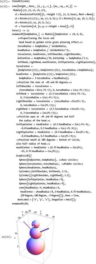In 7.6 Combining 2D Contours with 3D Plots, a 3D plot and a 2D contour plot are combined to achieve a 3D plot with a 2D contour "shadow" underneath. Another example is 7.10 Displaying 3D Geometrical Shapes: RevolutionPlot3D is used to generate a cone to compensate for the lack of a Cone primitive in Mathematica 6 (Cone is built into Mathematica 7). Achieving these results involves sticking your head under the hood and, sometimes, doing quite a bit of trial and error, but the results are within reach once you have the general principles.

In 18.5 Compiling Functions to Improve Performance, I discuss how the attributes of 3D graphics can be controlled through stylesheets. If you intend to create publication-quality documents in Mathematica, you should familiarize yourself with stylesheets.

You want to graph one or more built-in or user-defined functions of two variables.

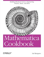
Use Plot3D with the function or functions to plot and two lists specifying the ranges for the independent variables.

As with most plots, you can provide multiple functions. However, 3D plots will become crowded quickly (Figure 7-1), so consider placing multiple plots side by side rather than trying to shoehorn everything into a single plot. With some functions and options, this is not an issue (Figure 7-1).

Figure 7-1. 3D plots of multiple functions

As you might suspect, Plot3D has a variety of options for customizing presentation. Here I use Complement to list only those options that differ from the 2D Plot function in 6.1 Plotting Functions in Cartesian Coordinates.

In[3]:=  Complement[First /@ Options[Plot3D], First /@ Options[Plot]]
Out[3]=  {AxesEdge, BoundaryStyle, Boxed, BoxRatios, BoxStyle, ControllerLinking,
          ControllerMethod, ControllerPath, FaceGrids, FaceGridsStyle,
          Lighting, NormalsFunction, RotationAction, SphericalRegion, ViewAngle,
          ViewCenter, ViewMatrix, ViewPoint, ViewRange, ViewVector, ViewVertical}

AxesEdge determines where the axes are drawn, and the default value of Automatic (Figure 7-2) usually gives good results. You can override the default by proving a specification of the form {{dir y, dir z},{dir x, dir z},{dir x, dir y}} where each dir i must be either +1 or -1, indicating whether axes are drawn on the edge of the box with a larger or smaller value of coordinate i, respectively (Figure 7-2).

Figure 7-2. Examples of AxesEdge option

BoundaryStyle allows you to stylize the edge of a plot surface.

Boxed, BoxRatios, and BoxStyle control the presence, proportions, and style of the edges surrounding 3D plots. Each of the plots in Figure 7-3 is of the same function. The differences are that Figure 7-3 is not boxed, Figure 7-3 is boxed with Automatic ratios, and Figure 7-3 and Figure 7-3 have specified ratios.

Figure 7-3. Examples of BoxRatios option

FaceGrids specifies grid lines to draw on the faces of the bounding box. You can specify All or specific faces using {x,y,z}, where two values are 0 and the third is either +1 (largest value) or -1 (smallest value). FaceGridsStyle allows you to stylize the grid to your liking.

ViewAngle, ViewCenter, ViewMatrix, ViewPoint, ViewRange, ViewVector, and ViewVertical are options that give you detailed control of the orientation of the plot. These are covered in 7.12 Controlling Viewing Geometry.

6.1 Plotting Functions in Cartesian Coordinates demonstrates Plot, which is the 2D counterpart to Plot3D.

You want to plot a surface with spherical radius r as a function of rotational angles θ (latitude) and ϕ (longitude).

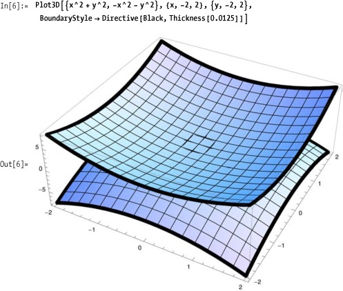
Use SphericalPlot3D when plotting one or more surfaces in spherical coordinates. Such plots most often arise in situations where there is some degree of rotational symmetry. For example, a sphere is fully symmetrical under all rotations and is trivially plotted using SphericalPlot3D as a constant radius.

You can plot multiple surfaces by providing a list of functions and leave holes in some of the surfaces by returning the symbol None for these regions.

Of course, you will probably use SphericalPlot3D to plot more interesting functions too.

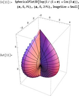
Use PlotStyle to achieve some dramatic effects. Applying the Opacity option is especially useful when specifying rotational angles greater than 2Pi radians; otherwise, the resulting interior surfaces would be hidden. Compare Figure 7-4 with Figure 7-4.

Figure 7-4. Effect of Opacity

See 7.4 Plotting 3D Surfaces Parametrically for the relationship between SphericalPlot3D and ParametricPlot3D.

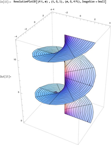
You want to visualize a surface generated via a revolution of a function or parametric curve around the z-axis.

Many common surfaces can be generated by revolving a 2D curve. The following examples illustrate the basic idea.

Revolve a parabola to create a bowl.

Revolve a vertical line at a constant distance from the center to create a cylinder.

Functions that incorporate the angle of revolution can create more exotic surfaces, such as the spiral shown here. Notice how the angle of revolution can be greater (or less) than 2Pi (one revolution).

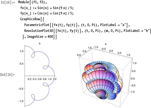
To get a feel for RevolutionPlot3D, plot the 2D parametric version of the equation next to the 3D revolution. It is fairly easy to see how the 180-degree rotation of the 2D curve around the y-axis in Figure 7-5 will yield the 3D surface shown in Figure 7-5.

Figure 7-5. Relationship between ParametricPlot and RevolutionPlot3D

RevolutionPlot3D was introduced in Mathematica 6. Prior to version 6, similar surfaces could be generated with ParametricPlot3D; however, the equations one needs to plot a specific surface using RevolutionPlot3D are often simpler and more intuitive than those used when plotting parametrically. Both of the following plots yield a torus, but the RevolutionPlot3D version is simpler.

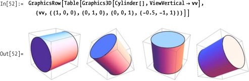
As of version 6, Mathematica did not have a RevolutionAxis option, which was in a legacy package called Graphics'SurfaceOfRevolution'. The effect could be emulated by swapping axes and using ViewVertical. Here I also use ViewPoint to compensate for the different default orientations of the two plotting functions, but that is not strictly necessary. The important aspect of the code that produces Figure 7-6 is the transposition of t and t^2 in RevolutionPlot3D.

Figure 7-6. Emulating SurfaceOfRevolution

(Note: RevolutionAxis was added in version 7.)

See discussion of ParametricPlot3D in 7.4 Plotting 3D Surfaces Parametrically.

See 7.12 Controlling Viewing Geometry for use of the geometry options ViewVertical and ViewPoint.

You want to plot a 3D curve or surface parameterized over a region defined by a range.

Here you plot a curve in 3D space by specifying a single variable u over the range [-Pi,Pi]. This creates the curve in 3D space, shown in Figure 7-7.

Figure 7-7. Curve in 3D space

Here you plot a surface in 3D space by specifying an area defined by variables u and v, yielding Figure 7-8.

Figure 7-8. Surface in 3D space

To get a better understanding of ParametricPlot3D, consider it as a generalization of the more specialized Plot3D. In Plot3D, the x and y coordinates always vary linearly over the range as it plots a specified function in the z-axis. This implies that you can mimic Plot3D using ParametricPlot (Figure 7-9). The only caveat is that you need to change the BoxRatios, which have different defaults in ParametricPlot3D.

Figure 7-9. Using ParametricPlot3D to emulate Plot3D

The relationship between ParametricPlot3D and SphericalPlot3D can be understood in terms of the following:

fx = f[θ,ϕ] sin θ cos ϕ

fy = f[θ,ϕ] sin θ sin ϕ

fz = f[θ,ϕ] cos θ

For example, if we pick f[ θ , ϕ ] to be the constant 1, both SphericalPlot3D and ParametricPlot3D give a sphere using this relationship.

You want to create a plot showing the surfaces where a function of three variables takes on a specific value (Figure 7-10).

Use ContourPlot3D with a function to produce evenly spaced contour surfaces for that function.

Figure 7-10. 3D contour plot example

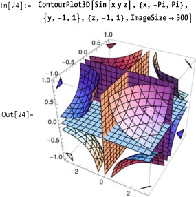
Use ContourPlot3D with an equivalence relation to plot the surface where the equivalence is satisfied. In Figure 7-11, ContourPlot3D shows the surface where the polynomial is equal to zero.

Figure 7-11. Surface where polynomial is zero

3D contour plots show surfaces of equal value. ContourPlot3D plots several equally spaced surfaces over the specified intervals. You use the option Contours → n, where n is an integer, to control the number of surfaces.

The 2D version ContourPlot is discussed in 7.6 Combining 2D Contours with 3D Plots.

You want to use a 2D contour plot to annotate the lower plane of a 3D plot.

Transform the 2D contour plot into a 3D graphic by adding a third z coordinate of constant value. Use Show to combine the new 3D graphic with a 3D plot.

You can apply the same technique to Plot3D. Here I use a larger PlotRange on the z-axis to provide room to see the contour. Using Opacity to add some translucence to the 3D plot also allows the contour plot to be better viewed.

You want to plot a 3D surface that includes only the points defined by a predicate.

Use the RegionFunction option with Plot3D, SphericalPlot3D, RevolutionPlot3D, ParametricPlot3D, and other 3D plots.

The parameters passed to a region function vary by plot type; these are listed in Table 7-1.

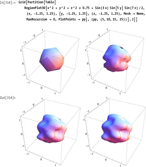
The region function can be used to create quite exotic effects, as demonstrated in Figure 7-12.

Figure 7-12. Effects of the RegionFunction option

You have a matrix of data points that you want to plot as heights, with possible interpolation of intermediate values.

Use ListPlot3D with InterpolationOrder→0 to plot distinct levels, InterpolationOrder→1 to join points with straight lines, and InterpolationOrder→2 or higher to create smoother surfaces.

In[31]:= SeedRandom[1000];
         data = RandomReal[{-10, 10}, {20, 20}];

3D list plots are often enhanced by use of a mesh. Here, in an example adapted from the Wolfram documentation, I show a plot of elevation of the state of Utah by latitude and longitude. The option MeshFunctions → {#3 &} uses the elevation data to specify the mesh giving contours (first image) that help visualize the elvation better than the default mesh (second image).

ListPointPlot3D is used to create 3D scatter plots.

You want to visualize regions where a predicate is satisfied.

RegionPlot takes a predicate of up to three variables. The predicate can use all of the relational operators (<, <=, >, >=, ==, !=) and logical connectives (&&, ||, Not).

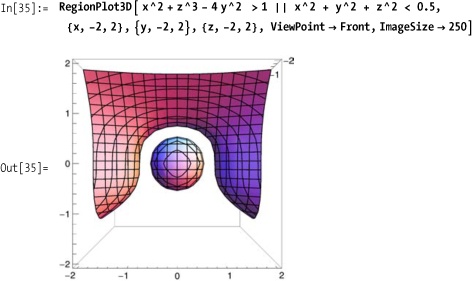
RegionPlot3D uses an adaptive algorithm that is based on the options PlotPoints and MaxReeursion. The default setting for each is Automatic, meaning Mathematica will pick what it thinks are appropriate values based on the predicate and ranges. The algorithm first samples using equally spaced points, and then subdivides those points based on MaxReeursions and the behavior of the predicate. It is possible for the algorithm to miss regions where the predicate is true. One way to gain confidence in the result is to plot with successively larger values for Plotpoints and MaxReeursion. However, of the two, PlotPoints usually has a more significant effect.

You want to create graphics that contain spheres, cylinders, polyhedra, and other 3D shapes.

Mathematica has 3D primitives: Cuboid, Sphere, Cylinder Line, Point, and Polygon.

A more mathematically inspired demonstration of graphics primitives is the Dandelin construction. Here one drops two spheres, one small and one large, into a cone such that the spheres do not touch. Consider a plane that slices through the cone tangent to the surface of both spheres. As you may know, a plane intersecting a cone traces an ellipse. What is remarkable is that the tangent points with the spheres are the foci of this ellipse. I adapt the construction from Stan Wagon’s Mathematica in Action (W.H. Freeman), upgrading it to take advantage of the advanced 3D features of Mathematica 6, such as Opacity and PointSize. I refer the reader to Wagon’s book for the derivation of the mathematics.

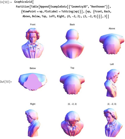
Mathematica can also deal with 3D graphics that are not necessarily of mathematical origin. You can demonstrate this using ExampleData.

You want to build a wireframe model or other structural models from an existing 3D plot.

The following solution was developed by Ulises Cervantes-Pimentel and Chris Carlson of Wolfram Research. As with 7.6 Combining 2D Contours with 3D Plots, the trick is to leverage Mathematica’s symbolic representation of 3D graphics and to perform transformations on that representation to yield the desired result.

You begin with the shape of interest. Here Chris Carlson was interested in an architectural model of a bubblelike structure. Note the use of the Mesh option, which is central to extracting the wireframe.

You can go directly to a wireframe by simply extracting the lines.

The solution was quite simple because the transformation was a simple extraction of graphics data that was already present. However, you can take this approach much further. Here Normal is used to force the Graphics3D object into a representation of low-level primitives, and Cases is used to extract the lines. However, this time the lines are transformed to polygons to create a box model.

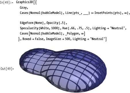
If your end goal was an architectural structure, the box model is no good. You need to open up the space. Here is an even more sophisticated transformation that turns the walls of the model into curved support beams.

As a final step, you may want to show how the structure would look if it were covered with a translucent covering. Here Mathematica’s sophisticated Lighting and Specularity options are used.

7.13 Controlling Lighting and Surface Properties covers Lighting and Specularity.

Chris Carlson gave a superb presentation at the 2009 International Mathematica User Conference (IMUC). This post on the Wolfram Blog covers a good portion of the talk: http://bit.ly/291CDE.

You want to control the placement of a simulated camera that determines viewing perspective of a 3D graphic.

Use the ViewPoint option to control the point in space from which a 3D object is to be viewed. Here I enumerate some of the possibilities.

Use the ViewCenter option to control the point that should appear as the center of the displayed image. The coordinates are scaled to the range [0,1].

Use the ViewVertical option to control which coordinates should be vertical.

For many users, combinations of ViewPoint, ViewCenter, and ViewVertical will create the initial spatial orientation of the 3D graphic that most suits your tastes or visual emphasis. However, there are additional options that are useful in some circumstances. ViewVector allows you to control the position and orientation of a simulated camera. ViewVector takes either a single vector that specifies the position of the camera that is pointed at ViewCenter or a pair of vectors that specify both the position of the camera and the center. ViewVector overrides ViewPoint and ViewCenter. To understand the concept of the camera, picture yourself looking through the camera as it moves around the stationary graphic.

Continuing with the camera metaphor, the option ViewAngle is analogous to zooming. The default view angle is 35 degrees. You can specify a specific angle or the symbol All, which will pick an angle that is sufficient to see everything.

You want to modulate lighting and surface characteristics to highlight important features or create artistic effects.

Mathematica provides quite sophisticated control of light via the options Lighting, Specularity, and Glow. The simplest settings for Lighting are Automatic, "Neutral", and None (Figure 7-13).

Figure 7-13. Examples of Lighting

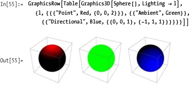
For more sophisticated control, you can specify combinations of ambient, directional, spot, and point light sources (Figure 7-14). Try the code on your own for the full effect.

Figure 7-14. Examples of Glow

Glow is the opposite of Lighting. It specifies the color of the surface itself. Glow is also different from an object’s color, as you can see in Figure 7-15. (However, Glow is not easily demonstrated in monochrome print. Please try the code on your own to see the effect.) Both the cylinder and the sphere have a green color, but the cylinder also has a green glow. There is no lighting, so only the cylinder appears bright because of Glow. Another way Glow differs from Lighting is that it does not affect surrounding objects, only the objects with Glow. In other words, a glowing object is not a light source in the Graphics3D domain.

Figure 7-15. Difference between Glow and color

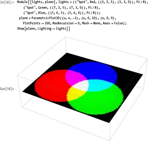
As you probably would expect from your experience with colored lights, Mathematica lighting follows the additive color model (refer to the online version of the following image to appreciate its full glory: http://bit.ly/xIgx7).

Lighting can be used as an option that applies to an entire graphic, but it also works as a graphics directive that applies to the objects that follow it within the same scope.

Specularity and Glow are strictly used as directives, although Specularity can be combined with Lighting.

The use cases covered in this recipe should satisfy most common uses of colored lighting, but if you are trying to achieve very specific lighting effects, you should consult the Mathematica documentation to explore the full range of forms Lighting, Specularity, and Glow can take and how they interact with color.

You want to scale, translate, or rotate graphics in 3D space.

Use Scale to stretch or shrink graphics.

Use Translate to move graphics in 3D space. Figure 7-16 presents four translations of a sphere that is originally constructed at the origin.

Figure 7-16. Examples of Translate

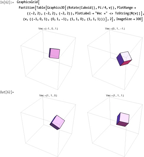
Use Rotate to change the orientation of graphics. Figure 7-17 rotates a cube through Pi/4 radians (45 degrees) but uses different vectors to define the rotation axis.

Figure 7-17. Examples of Rotate

In addition to the primitive transformations shown in the solution, Mathematica provides support for transformation matrices and symbolic transformation functions. Matrices include RotationMatrix, ScalingMatrix, ShearingMatrix, and ReflectionMatrix. The transformation functions are RotationTransform, TranslationTransform, ScalingTransform, ShearingTransform, ReflectionTransform, RescalingTransform, AffineTransform, and LinearFractional Transform. A smattering of examples is given here. Transformations work in conjunction with the function GeometricTransformation, which takes a graphic and either a transformation or a matrix.

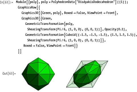
ShearingTransform[θ,v,n] is an area or volume preserving transformation that adds a slant, also known as a shear, to a graphic. Shear is specified in terms of an angle θ along a vector v and normal to a second vector n. Figure 7-18 shows a polyhedron in its original state followed by a shear transform. A translucent cube is also transformed to give a sense of the angles.

Figure 7-18. Example of ShearingTransform

You want to investigate the characteristics of various polyhedra.

Mathematica 6 includes PolyhedronData, which is effectively an embedded database of polyhedra attributes. Apropos to this chapter, PolyhedronData contains the 3D graphics data for a variety of common and exotic polyhedra. If you call PolyhedronData[] with no arguments, it returns a list of all polyhedra it has information about.

If you call PolyhedronData[poly], where poly is the name of the polyhedron, it will return the graphic. The code given here creates a labeled grid of a random selection of 20 polyhedra known to Mathematica 7. Here StringSplit uses a regular expression to parse the names on CamelCase boundaries and inserts a new line so the names fit inside the grid cells.

PolyhedraData contains a treasure trove of polyhedra information. In the solution we demonstrate how to extract graphics by name. Here we show the input form of a cube.

   In[66]:=  PolyhedronData["Cube"] // InputForm
Out[66]//InputForm=
             Graphics3D[GraphicsComplex[{{-1/2, -1/2, -1/2}, {-1/2, -1/2, 1/2}, {-1/2,
             1/2, -1/2}, {-1/2, 1/2, 1/2}, {1/2, -1/2, -1/2},
                {1/2, -1/2, 1/2}, {1/2, 1/2, -1/2}, {1/2, 1/2, 1/2}}, Polygon[{{8, 4, 2,
             6}, {8, 6, 5, 7}, {8, 7, 3, 4}, {4, 3, 1, 2},
                 {1, 3, 7, 5}, {2, 1, 5, 6}}]]]

The solution also exploits the ability to list all the polyhedra by providing no arguments. The solution used the first 20, but there are many more, as you can see.

In[67]:=  Length[PolyhedronData[]]
Out[67]=  187

You can explore all of them with this little dynamic widget.

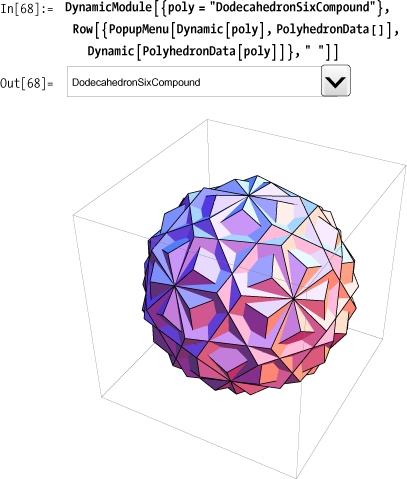
The polyhedra are grouped into classes. You can get a list of these classes or a list of the members of a particular class.

In[69]:=  PolyhedronData["Classes"]
Out[69]=  {Amphichiral, Antiprism, Archimedean, ArchimedeanDual, Chiral, Compound,
           Concave, Convex, Cuboid, Deltahedron, Dipyramid, Equilateral, Hypercube,
           Johnson, KeplerPoinsot, Orthotope, Platonic, Prism, Pyramid, Quasiregular,
           RectangularParallelepiped, Rhombohedron, Rigid, SelfDual, Shaky,
           Simplex, SpaceFilling, Stellation, Uniform, UniformDual, Zonohedron}

In[70]:=  PolyhedronData["Chiral"]
Out[70]=  {GyroelongatedPentagonalBicupola, GyroelongatedPentagonalBirotunda,
           GyroelongatedPentagonalCupolarotunda, GyroelongatedSquareBicupola,
           GyroelongatedTriangularBicupola, PentagonalHexecontahedron,
           PentagonalIcositetrahedron, SnubCube, SnubDodecahedron}

Polyhedra also have various properties, which you can list or use with a polyhedron to retrieve the value.

In[71]:=  PolyhedronData["Properties"]
Out[71]=  {AdjacentFaceIndices, AlternateNames, AlternateStandardNames, Amphichiral,
           Antiprism, Archimedean, ArchimedeanDual, Centroid, Chiral, Circumcenter,
           Circumradius, Circumsphere, Classes, Compound, Concave, Convex, Cuboid,
           DefaultOrientation, Deltahedron, DihedralAngleRules, DihedralAngles,
           Dipyramid, DualCompound, DualName, DualScale, EdgeCount, EdgeIndices,
           EdgeLengths, Edges, Equilateral, FaceCount, FaceCountRules, FaceIndices,
           Faces, GeneralizedDiameter, Hypercube, Image, Incenter, InertiaTensor,
           Information, Inradius, Insphere, Johnson, KeplerPoinsot, Midcenter,
           Midradius, Midsphere, Name, NetCoordinates, NetCount, NetEdgeIndices,
           NetEdges, NetFaceIndices, NetFaces, NetImage, NotationRules,
           Orientations, Orthotope, Platonic, PolyhedronIndices, Prism, Pyramid,
           Quasiregular, RectangularParallelepiped, RegionFunction, Rhombohedron,
           Rigid, SchlaefliSymbol, SelfDual, Shaky, Simplex, SkeletonCoordinates,
           SkeletonGraphName, SkeletonImage, SkeletonRules, SpaceFilling,
           StandardName, StandardNames, Stellation, StellationCount, SurfaceArea,
           SymmetryGroupString, Uniform, UniformDual, VertexCoordinates,
           VertexCount, VertexIndices, Volume, WythoffSymbol, Zonohedron}

In[72]:=  PolyhedronData["GyroelongatedPentagonalBicupola", "VertexCount"]
Out[72]=  30

Skeletal images show the polygons in terms of connected graphs.

NetImage is my favorite aspect of PolyhedronData because it shows how to make a cutout that can be folded into an actual 3D model of the named polyhedron. My kids like this one, too, although I have to do all the tedious parts!

GraphData, KnotData, and LatticeData are equally cool graphical data sources that you can explore on your own. Refer to the Mathematica documentation.

You have 3D data from another application that you would like to view or manipulate within Mathematica.

Mathematica 6 can import several popular 3D graphics formats, including Drawing Exchange Format (DXF) produced by AutoCAD and other CAD packages.

Mathematica’s symbolic representation makes it possible to manipulate imported graphics via pattern matching.

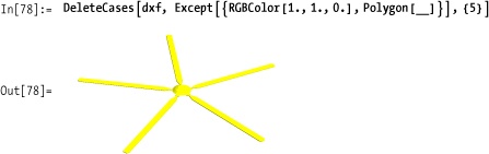
You can change colors and directives.

You can extract elements based on properties. Here we delete all nonyellow polygons (i.e., all but the rotor).

You can emphasize the component polygons by shrinking each toward its center and changing all colors to dark gray.