Mathematica uses the function Import to load images into a format suitable for processing and display within the frontend. When you use Import on an image file in versions of Mathematica prior to 7, you get a Graphics object that typically contains a single Mathematica graphics primitive called Raster. A Raster represents a 2D array of grayscale or color cells. A gray cell value will be a single number; a color cell value will be three or four numbers. An option called ColorFunction tells Mathematica how to map the cell values to display colors. Typical encodings are RGBColor, GrayLevel, and Hue. Most of the recipes in this chapter deal with grayscale images; however, the first recipe shows you how to transform red-greenblue (RGB) images to other encodings that are appropriate for the kinds of algorithms in these recipes.

As of version 7, Mathematica images have their own representation, called Image, which is distinct from Graphics (although you can request the older format for backward compatibility using "Graphic" with Import). To make these recipes compatible to both versions 6 and 7, I use the following functions throughout this chapter. However, in some recipes these are not sufficient because the code assumed Graphics form when recreating the image for display, and hence, expected Graphics options to be present in the imported version.

In[18]:=  Clear[getImgData, getImgRange, getImgDim, rasterReplace]

          getImgData[img_Graphics] := img[[1, 1]]
          getImgData[img_Image] := Reverse[ImageData[img, "Byte"]]

          getImgRange[img_Graphics]  := img[[1, 3]]
          getImgRange[img_Image] := Module[{},
            Switch[ImageType[img],  "Bit",{0, 1}, "Byte",
             {0, 255},"Bit16", {0, 65 535},"Real", {0.0, 1.0}]]

          getImgDim[img_Graphics] := img[[1, 2, 2]] -img[[1, 2, 1]]
          getImgDim[img_Image] := ImageDimensions[img]
          getImgCoord[img_Graphics] := img [[1, 2]]
          getImgCoord[img_Image]  := {{0, 0}, getImgDim[img]}

          rasterReplace[img_Graphics, raster_List, opts___] :=
          Graphics[Raster[raster, img[[1, 2]], opts, Sequence@@Options[img[[1]]]],
           Sequence@@Options[img]]

          rasterReplace[img_Image, raster_List, opts___]  :=
           Image[raster, img[[2]], opts, Sequence@@Options[img]]

Most of this chapter was originally written prior to the release of Mathematica 7, which introduced many native functions for image processing. After the release of version 7, I added content and augmented some of the recipes. However, I still left most of the custom algorithms intact, rather than just rewrite everything in terms of the built-in constructs. As I stated previously, I believe image-processing algorithms are interesting in their own right. The Mathematica 7 functions are very easy to use; if you want to sharpen an image, for example, use Sharpen and you are done. However, if you want to understand the mathematics, see 8.5 Sharpening Images Using Laplacian Transforms or 8.6 Sharpening and Smoothing with Fourier Transforms. In some recipes, I simply refer you to the appropriate Mathematica function in the See Also section. There are some common image transformations that are not covered in this chapter, but most are easily implemented and are native to Mathematica 7. If you need to crop, pad, rotate, and so on, you will want to upgrade to version 7, which has ImageCrop, ImagePad, ImageResize, ImageTake, and ImageRotate.

The recipes in this chapter draw heavily on Rafael C. Gonzalez and Richard E. Woods’s Digital Image Processing, Second Edition (Addison-Wesley). This is one of the classic texts in the field, and any individual who has a serious interest in image processing should own this text. Although I relied on the second edition, I would recommend buying the latest (third) edition, published by Prentice Hall in 2008.

If you have never worked with images in Mathematica, consult the documentation and experiment with the functions Import, Graphics, and Raster before diving into these recipes.

You want to extract information from one or more image files for manipulation by Mathematica or for combining into a new image.

Use the two-argument version of the Import function to selectively import data from an image file. Using Import with a PNG, GIF, TIFF, BMP, or other supported image format will import the image and display it in the Mathematica frontend. However, sometimes you might want to extract a subset of the image data for manipulation rather than display. What information can you extract? This is answered using a second argument of "Elements".

In[200]:=  Import[FileNameJoin[
             {NotebookDirectory[], "..", "images", "truck.jpg"}], "Elements"]
Out[200]=  {Aperture, BitDepth, CameraTopOrientation, ColorMap, ColorSpace, Data,
            DataType, Date, Exposure, FocalLength, Graphics, GrayLevels, Image,
            ImageSize, ISOSpeed, Manufacturer, Model, RawData, RGBColorArray}

Note that not every image will provide the same level of information. The image format and the device that produced the image determine which elements are available.

In[201]:=  Import[FileNameJoin[
             {NotebookDirectory[], "..", "images", "mechanism1.png"}], "Elements"]
Out[201]=  {BitDepth, ColorSpace, Data, DataType,
            Graphics, GrayLevels, Image, ImageSize, RGBColorArray}

Once you know which elements are available, you can extract them by name.

In[202]:=  Import[FileNameJoin[
             {NotebookDirectory[], "..", "images", "truck.jpg"}], "BitDepth"]
Out[202]=  8

Note that an image element might be supported but not available, in which case Import will return None.

In[203]:=  Import[
            FileNameJoin[{NotebookDirectory[], "..", "images", "truck.jpg"}], "Model"]
Out[203]=  None

However, if you ask for the value of an element that is not supported, Import will fail.

From an image processing point of view, the elements you will most likely extract are "Graphics", "Gray Levels", "Data", and "RGBColorArray". The "Graphics" element is the default element for an image file. It extracts the image in a format suitable for immediate display in the frontend.

Note, if you want to extract the "Graphics" format without displaying it, terminate the expression with a semicolon.

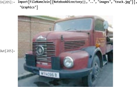
In[206]:=  image = Import[FileNameJoin[
                {NotebookDirectory[], "..", "images", "truck.jpg"}], "Graphics"];

The "GrayLevels" element will convert color image data to gray level data. That is, it will return a 2D array of pixel gray values in the range 0 (black) to 1 (white). Here I use Short to only show a few of the gray level values.

  In[207]:=  Short [Import[FileNameJoin[
                {NotebookDirectory[], "..", "images", "truck.jpg"}], "GrayLevels"], 6]
Out[207]//Short=
             {{0.283235, 0.330294, 0.270298, 0.242804, 0.227118, 0.190608,
               0.190608, 0.161494, 0.181102, 0.156357, 0.21518, 0.322149, 0.388816,
               0.446467, 0.524855, 0.576922, 0.620016, 0.646208, <<125>>,
               0.980071, 0.988663, 0.980373, 0.981588, 0.98551, 0.984592, 0.984592,
               0.984122, 0.972357, 0.985016, 0.985016, 0.984973, 0.984078,
               0.984078, 0.984592, 0.984592, 0.983698}, <<118>>, {<<1>>}}

The "Data" element will extract the image pixel data as it is stored in the image file. The format of the data will vary depending on the image type, but typically it will be a matrix of RGB triplets for a color image and gray values for a grayscale image both in the range [0,255].

  In[208]:=  Short[Import[FileNameJoin[
                {NotebookDirectory[], "..", "images", "truck.jpg"}], "Data"], 6]
Out[208]//Short=
             {{{86, 67, 63}, {98, 79, 75}, {82, 64, 60},  {73, 58, 53}, {69, 54, 49},
               {57, 46, 40}, {57, 46, 40}, {47, 40, 32},  {52, 45, 37}, {43, 40, 31},
               {58, 55, 46}, {82, 84, 73}, {99, 101, 90}, {113, 116, 105}, {131, 137, 125},
               {141, 152, 138}, {150, 164, 149}, {152, 173, 156}, {150, 175, 156},
               {141, 168, 149}, {136, 160, 144}, {142, 165, 149}, {149, 169, 157},
               {155, 173, 161}, {146, 163, 153}, {145, 165, 154}, {146, 167, 158},
               <<107>>, {246, 245, 241}, {250, 249, 245}, {255, 255, 251},
               {255, 255, 251}, {249, 251, 248}, {248, 250, 247}, {247, 251, 252},
               {249, 253, 254}, {248, 252, 255}, {247, 251, 252}, {248, 255, 248},
               {246, 253, 245}, {249, 252, 245}, {250, 253, 246}, {252, 251, 249},
               {252, 251, 249}, {254, 249, 253}, {251, 246, 250}, {254, 249, 255},
               {254, 249, 255}, {252, 250, 255}, {252, 250, 253}, {252, 250, 253},
               {252, 251, 249}, {252, 251, 249}, {252, 251, 247}}, <<118>>, {<<1>>}}

  In[209]:=  Short[Import[FileNameJoin[
                 {NotebookDirectory[], "..", "images", "truck.jpg"}], "RGBColorArray"], 6]
Out[209]//Short=
              {{RGBColor[0.337255, 0.262745, 0.247059],
                RGBColor[0.384314, 0.309804, 0.294118],
                RGBColor[0.321569, 0.25098, 0.235294],
                RGBColor[0.286275, 0.227451, 0.207843],
                RGBColor[0.270588, 0.211765, 0.192157],
                <<150>>, RGBColor[0.988235, 0.980392, 0.992157],
                RGBColor[0.988235, 0.980392, 0.992157],
                RGBColor[0.988235, 0.984314, 0.976471],
                RGBColor[0.988235, 0.984314, 0.976471],
                RGBColor[0.988235, 0.984314, 0.968627]}, <<119>>}

More details can be found in the Mathematica documentation for Import and the formats JPEG, TIFF, BMP, PNG, and GIF.

You have an image that is represented in RGB but most image-processing algorithms demand the hue-saturation-value (HSV) color space model.

The solution starts with defining some primitives to compute Hue, Saturation, and Value from Red, Green, and Blue intensities.

The HSV color model is often depicted geometrically as a cone (see http://en.wikipedia.org/wiki/Image:HSV_cone.png). The hue can be thought of as the angle of a vector rotating around the center, with angles close to 0 degrees corresponding to red and increasing angles moving through the rainbow out to violet and returning again to red. To simplify the math, we first scale the standard RGB values that range from 0 to 255 to values that range between 0 and 1. Mathematically speaking, you compute hue by finding which two of the three scaled RGB color intensities dominate and then using their difference to compute an angular offset from a starting angle determined by the third (least dominant) color. Here you divide the circle into six regions (red, orange, yellow, green, blue, violet) with i specifying the start region and f acting as a factor determining the offset from i. This value is scaled by the difference between the most dominant (rgbMax) and least dominant (rgbMin) color to yield a value between 0 and 6. Finally you divide by 6 to get a value for hue in the range [0,1].

In[210]:=  HueValue[r_Integer, g_Integer, b_Integer]  :=
            HueValue2[r /255.0, g /255.0, b/255.0]
           HueValue2[r_ /; r ≤1, g_/; g ≤1, b_/; b ≤1]  :=
            Module[{minRGB = Min[r, g, b], maxRGB =Max[r, g, b], f, i},
             Which[maxRGB == minRGB, Return[0],
              minRGB == r, f = g - b; i = 3,
              minRGB == g, f = b - r; i = 5,
              minRGB == b, f = r - g; i = 1];
             (i - f/(maxRGB -minRGB))/6]

Saturation is a measure of the purity of the hue. Highly saturated colors are dominated by a single color, whereas low saturation yields colors that are more muted. Geometrically, saturation is depicted as the distance from the center to the edge of the HSV cone. Mathematically, saturation is the difference between the most dominant and least dominant color scaled by the most dominant. Again, you scale RGB integer values to the range [0,1].

In[212]:=  SatValue[r_Integer, g_Integer, b_Integer] :=
            SatValue2[r /255.0, g/ 255.0, b/255.0]
           SatValue2[r_ /; r ≤1, g_/; g ≤1, b_/; b ≤1] :=
            Module[{minRGB = Min[r, g, b], maxRGB = Max[r, g, b]},
             If[maxRGB > 0,(maxRGB - minRGB)/ maxRGB, 0]]

The third component of the HSV triplet is the value, which is also known as brightness (HSV is sometimes referred to as HSB). The brightness is the simplest to compute since it is simply the value of the most dominant RGB value scaled to the range [0,1]. Geometrically, the value is the distance from the apex (dark) of the HSV cone to the base (bright).

In[214]:= BrightValue[r_Integer, g_Integer, b_Integer] := Max[r, g, b] /255.0

Given these primitives, it becomes a relatively simple matter to translate an image from RGB space to HSV space. But before you can do this, you need to understand how Mathematica represents imported images. The applicable function is called Raster, and it depicts a rectangular region of color or gray level cells. See the Discussion section for more information on Raster. The goal is to transform the RGB color cells to HSV color cells. An easy way to do that is to linearize the 2D grid into a linear array and then use the techniques from 2.1 Mapping Functions with More Than One Argument to transform this RGB array into an HSV array. To get everything back to a 2D grid, we use the Partition function with information from the original image to get the proper width and height. To get HSV images to display properly, we tell Mathematica to use Hue as the ColorFunction. Finally, we copy options from the original graphic to the new graphic, which requires a sequence rather than a list.

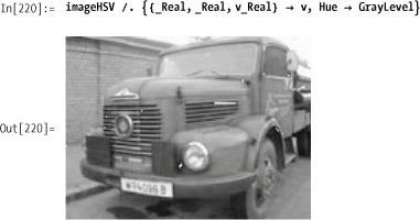
These two images of the red truck look identical, but we can see they have a very different internal representation by inspecting a portion of each Raster.

  In[218]:=  Short[getImgData[image][[1]], 3]
Out[218]//Short=
              {{104, 122, 142}, {99, 117, 137}, {94, 112, 132},
               {94, 112,  132}, {98, 119, 138}, {104, 125, 144}, {106, 127, 146},
               {106, 127, 146}, {101, 124, 142}, {101, 124, 142}, {100, 123, 141},
               {99, 122, 140}, {95, 121, 138}, <<134>>, {94, 116, 130},
               {92, 114, 128}, {92, 114, 128}, {93, 115, 129}, {95, 117, 131},
               {99, 121, 135}, {98, 120, 134}, {98, 120, 134}, {98, 120, 134},
               {99, 121, 135}, {101, 123, 137}, {103, 125, 139}, {104, 126, 140}}

  In[219]:=  Short[getImgData[imageHSV][[1]], 3]
Out[219]//Short=
              {{0.587719, 0.267606, 0.556863}, {0.587719, 0.277372, 0.537255},
               {0.587719, 0.287879, 0.517647}, <<155>>,
               {0.564815, 0.258993, 0.545098}, {0.564815, 0.257143, 0.54902}}

The major color spaces in popular use are RGB, HSV, and cyan-magenta-yellowblack (CMYK). RGB is the most common format because it maps directly onto display technology. The problem with RGB is that it is not very good for image analysis because colors that are close in perceptual space are not grouped together in RGB space. CMYK is most often used in printing. HSV is popular in image processing applications because the mathematical distance between the colors is more closely aligned with human judgments, yielding a closer approximation to human perception of color. Another advantage of HSV is that one can immediately convert from color to grayscale by discarding the hue and saturation components and retaining the value component.

Doing image processing in Mathematica requires familiarity with the Raster graphics primitive. When an image is imported from a JPEG, BMP, or GIF file, it will be represented as an RGB or grayscale Raster with cell values ranging from 0 through 255. The ColorFunction will be RGBColor for color image and GrayLevel for grayscale images. There are several forms of the Raster function, but the form you will typically encounter in image processing is Raster[array, dimensions, scale, ColorFunction → function], where array is a 2D array of integers or RGB triplets, dimensions defines a rectangle of the form {{xmin,ymin}, {xmax,ymax}}, scale specifies the minimum and maximum values in the array (typically {0,255}), and function is either GrayLevel or RGBColor. A good way to test algorithms is to mathematically create rasters so you have controlled test cases.

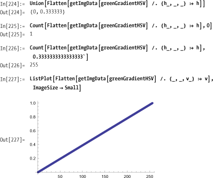
For example, the following is a green gradient in RGB space that varies from black in the lower left corner to bright green in the upper right. (Of course, you’ll need to try the code yourself to view the color effects.)

In HSV space, we expect the hue coordinate to be a constant (1/3) with the exception of the black corner element. The saturation should also be constant and the brightness values should form a straight line when plotted. This is easy to check.

In Mathematica 7, use ColorConvert (see the documentation center: http://bit.ly/irShF ).

Wikipedia has several very approachable articles on color models. See http://bit.ly/IWvVW , http://bit.ly/2DZAhY , http://bit.ly/3jawwr , and http://bit.ly/2qHxrI .

Color renderings of the images in this chapter can be found at http://bit.ly/xIgx7 or http://www.mathematicacookbook.com .

You have an image that is too dark or too light and you would like to increase contrast.

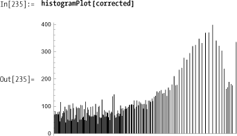
You obtain the histogram of a grayscale image using BinCounts on the flattened raster matrix. If an image has poor contrast, you will see that the histogram is skewed when you plot the histogram using BarChart.

Histogram equalization works by using the image distribution to derive a transformation function that will always yield a more uniform distribution of gray levels despite the shape of the input image’s distribution. The solution below will work on any grayscale image but is not very efficient. I’ll implement a more efficient solution in the Discussion section and also cover theory that explains why this transformation works.

Note how the histogram of the corrected image is more spread out than the input.

The theory behind automatic histogram equalization is based on probability theory. View the gray levels of an image as a random variable in the interval [0,1]. It is clear that grayscale ranges in the [0,255] range can be scaled to [0,1] simply by dividing by 255. Let pr[r] denote the probability density function (PDF) of the input image. Let ps[s] denote the desired PDF of the output image. In this case, we want ps[s] to be uniform. Let T[r] denote the transformation function applied to the input r to produce output s with PDF ps[s]. We want T[r] to be a single-valued monotonically increasing function. Single valued is necessary so that the inverse exists; monotonic prevents the transformation from inverting gray levels. We also want T[r] to have range [0,1]. Given these conditions, we know from probability that the transformed PDF is related to the original PDF by:

In the solution, we used the discrete form of the cumulative density function (CDF) as T[r]. The continuous form of the CDF is

By substitution, we obtain

We can ask Mathematica to evaluate this derivative for us by entering it in Mathematica syntax.

By substitution into the original equation, we get

Since the probabilities are always positive, we can remove the absolute value to prove that

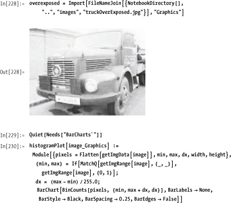
s[s] = 1

This means that the PDF of s is 1; hence, we have a uniform distribution. This demonstrates that in the continuous case, using the CDF as a transformation always yields a uniform distribution regardless of the characteristics of the input PDF. Of course, these results for the continuous domain do not translate exactly to the discrete domain, but it suggests that the discrete CDF will tend to shift gray levels to a more uniform range. To gain some deeper insight, you can plot the transformation function obtained from the histogram of the overexposed image.

This shows that all but the brightest levels will be mapped to darker levels; thus an overly bright image will tend to be darkened. The opposite will occur for an overly dark (underexposed) input image.

The nature of the transformation function leads to an obvious optimization: a precomputed lookup table computed in a single pass using FoldList. This lookup table can be used as the transformation function. This produces an O(nPixels) algorithm from our original O(nLevels * nPixels).

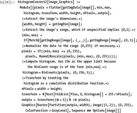
As you can see, there is a two-orders-of-magnitude performance improvement for histogramCorrect2.

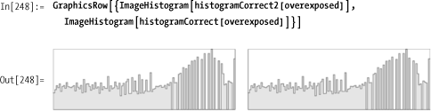
Here are the histograms from each for comparison.

Mathematica 7 has the native function ImageHistogram for plotting an image’s histogram.

8.3 Enhancing Images Using Histogram Equalization shows how histograms can be used to match one image’s contrast to that of a reference image.

You need to transform the gray levels of an image to match another image’s histogram.

To match a histogram of one image to another, you produce the equalization transform of the input image as in 8.1 Extracting Image Information. You then produce the equalization transform of the target image, and from that and the input transform, derive the final specification transform. Next, map the input through the specification transform to yield an image that approaches the target image’s histogram. Since you need to build the equalization transform for each image, it makes sense to factor that logic into a separate function. Here I call it buildEqualizationMap. You will recognize the basic logic from 8.2 Converting Images from RGB Color Space to HSV Color Space.

In[249]:=  buildEqualizationMap[image_Graphics]  :=
            Module[{pixels, min, max, histogram, width, height, nPixels},
             pixels=Flatten[getImgData[image]];
             {min, max} = If[MatchQ[getImgRange[image], {_, _}],
               getImgRange[image], {0, 1}];
             pixels = If[{min, max} == {0, 255}, pixels,
               Rescale[pixels, {min, max}, {0, 255}]];
             nPixels= Length[pixels];
             histogram=BinCounts[pixels, {0, 256, 1}];
             N[Rest[FoldList[Plus, 0, histogram]] * 255/nPixels]]

The main function must build the map for each image and use those maps to derive the final transformation (here it is called specMap). The logic underlying the derivation of specMap is explained in the Discussion section and was adapted from work by Nikos Drakos and Ross Moore (refer to the See Also section). Here we take advantage of Reap and Sow to build up specMap incrementally without the overhead of Append.

To demonstrate histogramSpecification, I’ll synthesize two raster images with different grayscale levels, using one as the input and the other as the target. In 8.4 Correcting Images Using Histogram Specification there is a much less contrived example of this algorithm’s application.

Here you can see the darker test image has been shifted toward the lighter target image.

In 8.2 Converting Images from RGB Color Space to HSV Color Space we saw how histograms can be used to automatically equalize an image’s contrast. However, sometimes it is preferable to equalize based on a reference histogram rather than a uniform distribution. This often arises when transformations are applied to an image and have side effects that reduce contrast—side effects we wish to undo by shifting the image back to the grayscale distribution of the original image (see 8.4 Correcting Images Using Histogram Specification).

To appreciate the theory behind the solution, imagine an image that has a uniform grayscale distribution. Suppose you want to transform this hypothetical image to the distribution of the target image. How could you produce such a transformation? You already know how to transform the target image to a uniform distribution (8.2 Converting Images from RGB Color Space to HSV Color Space); it follows that the inverse of this transformation will take the uniform distribution back to the target distribution. If we had this inverse distribution, we could proceed as follows:

The key to the solution is finding the inverse. Since you are working in a discrete domain, you cannot hope to find the exact inverse, but you can approximate the inverse by flipping the targetMap, taking the minimal unique values, and filling in missing values with the next closest higher entry. The function inverseEqualizationMap shown here will build such an inverse from an image. However, if you inspect the code in histogramSpecification, you’ll see that for efficiency the inverse is never built, but rather it computes the specification map directly using specificationMap from the input and target equalization transformations (inputMap and targetMap).

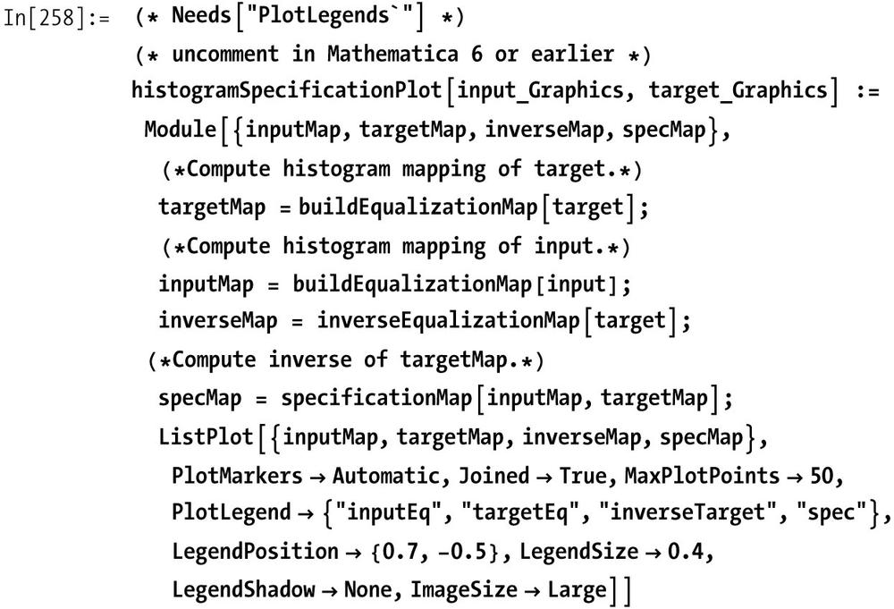
We can gain some insight into this process by creating a function histogram-SpecificationPlot, which plots the input transform, target transform, target inverse, and the resulting histogram specification transform. These plots show how input gray levels are mapped to output gray levels. If you are not convinced that specificationMap gives the desired transformation, replace the plot of specMap with inverseMap[#]& /@ inputMap to see that it yields the same plot.

The theory behind histogram specification can be found in Gonzalez and Woods, but for the implementation, I am indebted to Professor Ruye Wang’s lecture notes, available at http://bit.ly/4oSglp . Wang’s lecture contains information originally published by Nikos Drakos (University of Leeds) and Ross Moore (Macquarie University, Sydney).

You want to emphasize edges in the image and make them easier for the eye to pick out. You want to work in the spatial domain.

This transformation is performed as a convolution of the image with one of the Laplacian kernels in Figure 8-1.

Figure 8-1. Laplacian kernels

The built-in function ListConvolve makes it easy to implement image convolution in Mathematica. The only caveat is that by default, ListConvolve returns a matrix that is smaller than the input. However, you can specify a cyclic convolution by passing a third parameter of 1 to ListConvolve to make the output size match the input size. Refer to the ListConvolve Mathematica documentation for clarification.

Here we want to see more fine detail of the craters in an image of the moon. The transform achieves this but we lose contrast. We can readjust contrast using the histogramSpecification algorithm from 8.3 Enhancing Images Using Histogram Equalization.

The Laplacian of a continuous 2D function is given as

This equation is not useful for image processing and must be converted to discrete form. A common way to do this is to express each component in finite difference form and sum the result.

This leads to the convolution kernel shown in Figure 8-2. To improve results in the diagonal directions, one can add terms for each of the four diagonal components—for example, f(x+l,y+l)—each which contributes a negative f(x,y) term leading to the kernel in Figure 8-2. Equivalently, one can multiply each of these kernels by -1, with the sign of the center value determining whether you add or subtract the transformation from the input image to get the sharpened version. Since the operation is based on second derivatives, it creates a sharp response in areas of discontinuities and a shallow response around more slowly varying gray levels. This can be seen by viewing the output of the transformation directly (i.e., before it is added to the input image).

Figure 8-2. Convolution kernels

In Mathematica 7, you can use Sharpen ( http://bit.ly/2rutpn ).

You want to emphasize either the low or high frequency characteristics of an image.

Fourier-based image processing in Mathematica is particularly easy to implement since it has the native function Fourier, which implements a high-quality version of the Fast Fourier Transform (FFT). The basic steps of Fourier image processing are

The fourierFilter function is designed to work with a custom filter function. Here are some common functions found in the literature. See the Discussion section for more details.

In[11]:=  dist[u_, v_, rows_, cols_]  := Sqrt[(u-rows/2.)^2 + (v - cols/2.)^2]

In[12]:=  idealLowPass[u_, v_, rows_, cols_, d0_] :=
           If[dist[u, v, rows, cols]  ≤ d0, 1, 0]

In[13]:=  idealHighPass[u_, v_, rows_, cols_, d0_] :=
           If[dist[u, v, rows, cols]  ≤ d0, 0, 1]

In[14]:=  butterWorthLowPass[u_, v_, rows_, cols_, d0_, n_] :=
           1.0/(1.0 + (dist[u, v, rows, cols]/d0)^2 n)

One can use a low-pass filter for blurring an image. This might be done as a single stage of a multistage process applied to text that will be processed by OCR software. For example, blurring can diminish gaps in letters. This might be followed by a threshold transformation and other adjustments.

An important step in this algorithm is centering the zero frequency component of the transform. This allows filter functions to use the distance from the center as a function of increasing frequency. There are two ways to achieve centering. One way is to preprocess the image before it is transformed by multiplying it by the function (-1)x+y. This function produces a matrix of alternating values 1 and -1. This is the technique used in the solution.

Alternatively, one can postprocess the Fourier output by swapping quadrants using the quadSwap function.

I include both methods because you may encounter either of them in the literature. Gonzalez and Woods use the preprocessing technique, although I find the postprocessing technique easier to understand conceptually.

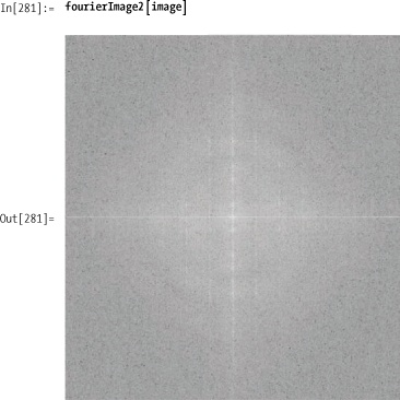
It is difficult to appreciate the meaning of complex images after they are mapped into the frequency domain. However, almost every image-processing text that discusses the Fourier transform will provide images of the transformation after centering. The fourierImage function below does this using quadSwap, whereas fourierImage2 uses (-1)x+y. You can see that they produce equivalent results. You’ll notice that each function maps Log[#+1] over the pixel values because Fourier transforms produce images with a much too large dynamic range.

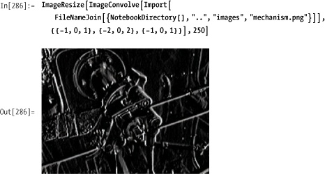
You want to detect boundaries between distinct objects in an image possibly as a preprocessing step to object recognition.

Two popular methods of edge detection are the Sobel and Laplacian of the Gaussian (LoG) algorithms. The Sobel is based on first-order derivatives that approximate the gradient. The LoG algorithm combines the second-order Laplacian that we used in 3.3 Determining Order Without Sorting with a Gaussian smoothing to reduce the sensitivity of the Laplacian to noise. See the Discussion section for further details. This implementation uses transformation rules that map intermediate gray levels to either white or black to emphasize the edges.

The edgeDetectSobel function provides the orientation optional parameter for extracting just the x edges {1,0}, just the y edges {0,1}, or both {1,1} (the default).

The edgeDetectLOG function provides a way to customize the kernel. See the Discussion section for criteria of appropriate kernels.

An edge is a set of connected pixels that lie on the boundary of two regions. Edges are local areas of discontinuity rather than more global regions. An ideal edge would have a sharp transition between two very different grayscale values; however, few realistic images will have edges that are so sharply defined. Typically an edge transition will be in the form of a ramp from one level to the next, possibly with some noise superimposed on the transition. See Gonzalez and Woods for some nice visualizations of these concepts.

Since edges are transitions, it is not surprising that methods of edge detection are based on mathematical derivatives. First derivatives of a noisy ramp will produce an approximate square wave transition along the length of the ramp. Second derivatives will form a spike at the start of the edge transition and one of opposite sign at the end.

The Sobel masks and Laplacian masks approximate first and second derivatives in the discrete domain. There are two masks in the first-derivative Sobel method. The first finds horizontal edges; the second finds vertical edges. The function edgeDetectSobel is written so that you can use the second parameter to emphasize both edges {1,1}, horizontal edges {1,0}, or vertical edges {0,1}.

The edgeDetectLOG functions uses a larger 5 × 5 mask to better approximate the Mexican hat response function sought by that transformation (large central peak, with rapid tapering off, followed by a gentle increase). This transformation creates finer lines but is more sensitive to image noise.

Mathematica 7 has ImageConvolve. Here is an example using a Sobel mask.

Given an initial training set of images, you want to find the best match of an input image to an image in the training set.

Here we show a solution that uses concepts from principal component analysis (PCA) and information theory to map a high-dimensional training set of images into a lower dimension such that the most significant features of the data are preserved. This allows new images to be classified in terms of the training set.

In[287]:=  (*Helper for vectorizing and scaling image data*)
           imageVector[image :(_Graphics| _Image)]  :=
            N[Rescale[Flatten[getImgData[image]]]]

           (*Computes eigenimage vectors, avg image vector,
           and eigenvectors of reduced M × M system
            where M is the number of training images*)
           eigenImageElements[images_List, frac_ : 0.5] :=
            Module[{imgMatrix = imageVector /@ images,
              imgMatrixAdj, imgAverage, eigenVecs},
             imgAverage = N[Total[imgMatrix]/Length[imgMatrix]];
             imgMatrixAdj = (# - imgAverage) & /@   imgMatrix;
             eigenVecs = Eigenvectors[Dot[imgMatrixAdj, Transpose[imgMatrixAdj]]];
             imgMatrixAdj =
              Dot[Take[eigenVecs, Ceiling[frac *Length[eigenVecs]]], imgMatrix];
             {imgMatrixAdj, imgAverage, eigenVecs}]

           (*Computes the eigenimages and
            average image from a set of training images*)
           eigenImages[images_List, frac_ : 0.5] :=
            Module[{eigenImages, imgAvg, dummy, img1  = images[[1]], width},
             {eigenImages, imgAvg, dummy}   = eigenImageElements[images, frac];
             width=getImgDim[img1][[1]];
             Graphics[Raster[Partition[Rescale[#], width], img1[[1, 2]], {0.0, 1.0}],
                 Options[img1]] & /@ Append[eigenImages, imgAvg]
            ]
           (*Computes a set of weight vectors for each input image,
           and acceptance threshold for matching new
            images based on the results from eigenImageElements*)
           eigenImageRecognitionElements[images_List, frac_ : 0.5]  :=
            Module[
             {eigenImages, imgAvg, dummy, weightVecs, thresholdVec, threshold},
             {eigenImages, imgAvg, dummy} = eigenImageElements[images, frac];
             weightVecs =
              Table[Dot[imageVector[images[[i]]] - imgAvg, eigenImages[[j]]],
                 {i, 1, Length[images]}, {j, 1, Length[eigenImages]}];
             thresholdVec = Table[Dot[imgAvg, eigenImages[[i]]],
                 {i, 1, Length[eigenImages]}];
             threshold = Min[EuclideanDistance[thresholdVec, #] & /@ weightVecs]/  2;
             EigenImageElements[{weightVecs, threshold, eigenImages, imgAvg}]]

           (*Given a training set, determines if a test image matches any image in
            the set and also returns the possible matches ranked best to worst*)
           eigenImageRecognition[images_List,
             testImage :(_Graphics | _Image), frac_ : 0.5] :=
            Module[{eigenImages, imgAvg, dummy, weightVecs, testVec,
              matchDistances, matchOrdering, match, thresholdVec, threshold},
             {weightVecs, threshold, eigenImages, imgAvg} =
              eigenImageRecognitionElements[images, frac][[1]];
             testVec = Table[Dot[imageVector[testImage] -imgAvg, eigenImages[[i]]],
               {i, 1, Length[eigenImages]}];
             matchDistances = EuclideanDistance[testVec, #] & / @ weightVecs;
             matchOrdering = Ordering[matchDistances];
             matchDistances = matchDistances[[matchOrdering]];
             {matchDistances[[1]]  ≤ threshold,
              Inner[List, matchOrdering, matchDistances, List]}
             ]
           (*This function is more efficient when many test images need to
            be matched since it allows you to compute the eigenImageElements
            once for the training set and reuse it for each test image.*)
           eigenImageRecognition[eigenImageElements_EigenImageElements,
             testImage : (_Graphics | _Image), frac_ : 0.5] :=
            Module[{eigenImages, imgAvg, dummy, weightVecs, testVec,
              matchDistances, matchOrdering, match, thresholdVec, threshold},
            {weightVecs, threshold, eigenImages, imgAvg} = eigenImageElements[[1]];
            testVec = Table[Dot[imageVector[testImage] -imgAvg, eigenImages[[i]]],
               {i, 1, Length[eigenImages]}];
             matchDistances = EuclideanDistance[testVec, #] & /@ weightVecs;
             matchOrdering = Ordering[matchDistances];
             matchDistances = matchDistances[[matchOrdering]];
             {matchDistances[[1]]  ≤ threshold,
              Inner[List, matchOrdering, matchDistances, List]}
            ]

I use a training set of faces obtained from the Yale Faces Database. These images were labeled "normal" in the database and were normalized manually in Photoshop to center the faces and equalize image dimensions.

In[293]:=  faces = Import[#, "Graphics"] &/@ FileNames[FileNameJoin[
                {NotebookDirectory[], "..", "images", "faces", "subject*.png"}]];

The solution is based on work performed by Matthew Turk and Alex Pentland at the MIT Media Laboratory. They were inspired by earlier work by L. Sirovich and M. Kirby for representing faces using PCA to efficiently encode face images. PCA is a technique for identifying patterns in data by highlighting similarities and differences. PCA is used to reduce high-dimensional data sets. It uses the most significant eigenvectors (those with the greatest eigenvalues) of a covariance matrix to project the high-dimensional data on a smaller dimensional subspace in terms of the eigenvectors.

In the case of image recognition, you start with a training set of images normalized to the same dimensions. For this example I used images from the Yale Face Database that I normalized to 180 × 240 pixels with the face centered.

The first step is to represent the images as vectors by flattening and normalizing the raster data. The helper function imageVector is used for that purpose. The vectors are then grouped into a matrix of 15 rows and 43,200 (180 × 240) columns and normalized by subtracting the average of all images from each image. If the solution used PCA directly, it would then need to generate a 43,200 × 43,200 covariance matrix and solve for the 43,200 eigensystem. Clearly this brute force attack is intractable. Rather, the solution takes advantage of the fact that in a system where the number of images (15) is much less than the number of data points (43,200), most eigenvalues will be zero. Hence, it takes an indirect approach of computing the eigenvectors of a smaller 15 × 15 matrix obtained from multiplying the image matrix by its transpose as explained in Turk and Pentland. A fraction (half by default) of these eigenvectors are then used to compute the eigenimages from the original image data. This work is encapsulated in the function eigenImageElements, which returns the eigenimages, the average image, and the computed eigenvectors of the smaller matrix. This prevents the need to recompute these values in other functions.

The function eigenImages is used to visualize the results. It returns a list of graphics containing each of the eigenimages plus the average image. Here we show all 16 (15 eigen + 1 average) images by setting frac to 1. The ghostlike quality is a standard feature of eigenimages of faces. Recalling that the lightest areas of a grayscale image represent the largest magnitudes, you can see the elements of each image that are emphasized. For example, the area around the cheek bones of the first image are the most significant.

The eigenimages can be used as a basis for image recognition by using the product of the eigenimages and the original images to form a vector of weights for each test image. The weights represent the contribution of eigenimage to the original image. Given these weight vectors, you can compute similar weights for an unknown image and use the Euclidean distance as a classification metric. If the distance is below a certain threshold, then a match is declared.

The test images are derived from some non-face images, some distortions of facial images, and other poses of the faces in the training set. The function eigenlmageRecognition returns a Boolean and a ranking list. The Boolean determines if the test image fell in the threshold of the training set. The threshold is computed using the av erage image distance. The ranking set ties the index to the image in the training set and the distance in order of increasing distance. This means the first entry is the best match to the training image.

The code that follows displays the best match in the training set that corresponds to the test image. If the threshold was not met, an X is superimposed on the image.

These results show a false positive for the second image in the first row, the first images in the second and third rows, and the fourth image in the third row. There is a false negative for the second image in the second row, meaning there was a correct match but it fell below the threshold. All other results are correct. This is pretty good considering the small size of the training set.

The images used here can be found at http://bit.ly/xlgx7 or http://www.mathematicacookbook.com . The original Yale Face Database can be found at http://bit.ly/52Igvb .

The original research of paper Eigenfaces for Recognition by Matthew Turk and Alex Pentland from the Journal of Cognitive Neuroscience (Volume 3, Number 1) can be found at http://bit.ly/70SSBw .

An excellent tutorial by Lindsay I. Smith on PCA can be found at http://bit.ly/6CJTWn .