
I’ve got the brains, you’ve got the looks Let’s make lots of money You’ve got the brawn, I’ve got the brains Let’s make lots of money
—Pet Shop Boys, "Opportunities (Let’s Make Lots of Money)"
Financial engineering (also known as computational finance) is the use of computers to create mathematical models and simulations that attempt to price financial instruments, model their sensitivity to changes in the market, hedge against these changes, and measure and manage risk. This is a high-stakes game, where there can be great reward for getting things right but even greater loss if you get things wrong. This became acutely evident during the financial crisis that started around July 2007. It might be tempting to conclude that attempts to bring mathematical rigor to the chaos of the market is foolhardy, but this would be like concluding that traditional engineering is foolhardy because a plane crashed or a bridge fell. Such failings are human failings, not mathematical ones. They only point to the need to use computational tools more diligently and more responsibly.
One goal for this chapter was to create a variety of recipes with a range of difficulties. This means that there are some recipes that may seem trivial and others that a novice might find difficult. Almost every recipe tries to demonstrate techniques that are unique to Mathematica; I hope readers of every skill level will take away techniques that they can apply to financial problems that interest them.
Mathematica has unique characteristics lacking in many
other tools commonly used in the financial industry. As of version 6,
Mathematica has integrated financial data that is essential to testing
your models. This is a big plus; having worked in the industry, I have
seen how hard it can be for quants (quantitative
analysts) to get data easily that is immediately usable. This may seem
counterintuitive; it seems that investment banks and hedge funds would
be swimming in data. They are, but you often must exert great effort to
access it because of technical, logistical, and political barriers.
14.1 Leveraging Mathematica’s Bundled Financial Data explains how
to use FinancialData to get access to
historical and delayed market data. Unfortunately, FinancialData is still incomplete. As of
version 7, it concentrates mainly on equities, commodities, and currency
data. There is nothing related to government, municipal, or corporate
bonds; options; or interest rates. Luckily, Mathematica will import data
from other sources; 14.2 Importing Financial Data from Websites shows an example of
that.
Another important feature of Mathematica is its ability to find
exact solutions using its unparalleled symbolic capabilities. Exact
solutions, when you can get them, overcome the errors and inaccuracies
introduced by numerical methods, especially around the boundaries of a
solution. For example, when computing Greeks it is advantageous if you
can compute a symbolic derivative (D)
rather than a numerical one (ND).
14.6 Black-Scholes for European Option Pricing shows how
the symbolic capabilities of Mathematica can be used to compute and
visualize the Greeks for European style options. See the introductory
sidebar on A Brief Introduction to Computational Finance for the
Nonquant
if this is all Greek to you!
Performance is important in financial engineering, and getting
Mathematica to perform well can be tricky for the novice. 14.8 Speeding Up NDSolve When Solving Black-Scholes and Other
PDEs, 14.9 Developing an Explicit Finite Difference Method for the
Black-Scholes Formula, and 14.10 Compiling an Implementation of Explicit Trinomial for Fast
Pricing of American Options show how to use
some of the optimized special functions that execute at machine speed
and how to use Compile to eliminate
the overhead of handwritten interpreted code. When writing numerically
intense financial functions, you should try to compile as much as
possible, but there are cases where functions cannot be compiled fully
and where doing so may influence results.
Finally, Mathematica has some of the best visualization tools for checking your models and developing an intuition for their behaviors across different regions of the solution. Almost every recipe includes 2D or 3D plots, but 14.12 Visualizing Trees for Interest-Rate Sensitive Instruments shows how you can use lower-level graphics primitives to create useful diagrams.
The classic text in this area is Options, Futures, and Other Derivatives by John C. Hull (Prentice Hall).
The Wilmott Journal and magazine discuss modern ideas in quantitative finance: http://bit.ly/rm9hO.
If you have more of a passing interest, Wikipedia has good definitions and basic explanations of most of the ideas discussed here.
An excellent book that teaches Mathematica programming in parallel with financial engineering is Computational Financial Mathematics Using Mathematica by Srdjan Stojanovic` (Springer).
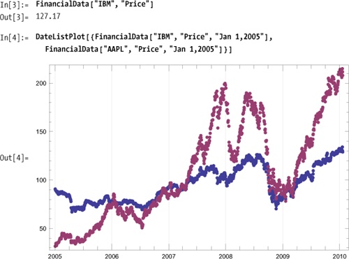
Use Mathematica’s curated financial data, FinancialData. This is a data source that
you can query to extract quite a variety of up-to-date data (15-minute
delayed and historical) on a variety of security types, what
Mathematica calls "Groups". To see
the available groups, execute the following. If this is the first time
you are doing this, you will see the status message "Initializing Financial Indices", and the
groups will display.
In[1]:=  FinancialData["Groups"]
Out[1]=  {Currencies, Exchanges, ExchangeTradedFunds,
          Futures, Indices, MutualFunds, Sectors, Stocks}
The next thing you will want to find is the available properties of the data.
In[2]:=  FinancialData["Properties"]
Out[2]=  {Ask, AskSize, Average200Day, Average50Day, AverageVolume3Month,
          Bid, BidSize, BookValuePerShare, Change, Change200Day, Change50Day,
          ChangeHigh52Week, ChangeLow52Week, CIK, Close, Company,
          CumulativeFractionalChange, CumulativeReturn, CUSIP, Dividend,
          DividendPerShare, DividendYield, EarningsPerShare, EBITDA, Exchange,
          FloatShares, ForwardEarnings, ForwardPERatio, FractionalChange,
          FractionalChange200Day, FractionalChange50Day, FractionalChangeHigh52Week,
          FractionalChangeLow52Week, High, High52Week, ISIN, LastTradeSize,
          LatestTrade, Lookup, Low, Low52Week, MarketCap, Name, Open, PEGRatio,
          PERatio, Price, PriceTarget, PriceToBookRatio, PriceToSalesRatio,
          QuarterForwardEarnings, Range, Range52Week, RawClose, RawHigh,
          RawLow, RawOpen, RawRange, Return, Sector, SEDOL, ShortRatio,
          SICCode, StandardName, Symbol, Volatility20Day, Volatility50Day,
          Volume, Website, YearEarningsEstimate, YearPERatioEstimate}
Now you can retrieve data for a specific symbol. By default, you will get the current price, but you can also ask for data from a specific date or within a date range.
FinancialData has a rich
interface that allows you to perform many types of queries. First,
let’s see how you can use the interface to find what is available.
Suppose you are curious to see what coverage there is for a specific
symbol.
In[5]:=  FinancialData["IBM", "Properties"]
Out[5]=  {Ask, AskSize, Average200Day, Average50Day, AverageVolume3Month,
          Bid, BidSize, BookValuePerShare, Change, Change200Day, Change50Day,
          ChangeHigh52Week, ChangeLow52Week, CIK, Close, Company,
          CumulativeFractionalChange, CumulativeReturn, CUSIP, Dividend,
          DividendPerShare, DividendYield, EarningsPerShare, EBITDA, Exchange,
          FloatShares, ForwardEarnings, ForwardPERatio, FractionalChange,
          FractionalChange200Day, FractionalChange50Day, FractionalChangeHigh52Week,
          FractionalChangeLow52Week, High, High52Week, ISIN, LastTradeSize,
          LatestTrade, Lookup, Low, Low52Week, MarketCap, Name, Open, PEGRatio,
          PERatio, Price, PriceTarget, PriceToBookRatio, PriceToSalesRatio,
          QuarterForwardEarnings, Range, Range52Week, RawClose, RawHigh,
          RawLow, RawOpen, RawRange, Return, Sector, SEDOL, ShortRatio,
          SICCode, StandardName, Symbol, Volatility20Day, Volatility50Day,
          Volume, Website, YearEarningsEstimate, YearPERatioEstimate}
One difficulty is that every security is not guaranteed to have
every property populated. There seem to be two possibilities when a
property is not present. You may get Missing["NotAvailable"] or you may get an
unevaluated expression like FinancialData["IBM",
"CumulativeFractionalChange"]. One way to see what
properties are populated and also get a sample of the associated data
is to execute the following (I elide the results with Short).
     In[6]:=  With[{sec ="IBM"},
                Select[
                 Table[{prop, FinancialData[sec, prop]},
                  {prop, FinancialData[sec, "Properties"]}],
                 FreeQ[#, {_, Missing["NotAvailable"] |
                     HoldPattern[FinancialData[__]]}] &]] // Short
Out[6]//Short=
             {{Average200Day, 122.097}, {Average50Day, 129.82}, <<54>>,
              {YearEarningsEstimate, 11.08}, {YearPERatioEstimate, 11.64}}
Let’s look at other types of financial data and see some of the additional capabilities that are provided. Industry sectors are especially useful for studying and comparing different industries’ performance.
In[7]:=  Length[FinancialData["Sectors"]]
Out[7]=  169
There are 169 sectors. Here I use a pattern to find those with the string "Service" in the name.
In[8]:=  Select[FinancialData["Sectors"], StringMatchQ[#, __ ~~"Service"~~__] &]
Out[8]=  {CommunicationsServicesNotElsewhere,
          LegalServices, MiscellaneousBusinessServices,
          MiscellaneousHealthAndAlliedServicesNot, OilNaturalGasFieldServices,
          RefrigerationServiceMachinery, ResearchDevelopmentAndTestingServices,
          TruckingAndCourierServicesExceptAir}
Given a sector, you can ask for its members. You can also use
"Members" with an index, such as
the S&P 500, or an exchange like the New York Stock Exchange
(NYSE). Here I pick 10 OilNaturalGasFieldServices members at
random.
 In[9]:=  RandomChoice[FinancialData["OilNaturalGasFieldServices", "Members"], 10]
 Out[9]=  {DE:HRL, PK:ONXC, PK:ASRPF, F:SJR,
           PK:VTHC, F:DG1, NYSE:WG, TO:POU, TO:POU, DE:DO1}

In[10]:=  Mean[Select[Quiet[FinancialData[#, "Price"] & /@
              FinancialData["OilNaturalGasFieldServices", "Members"]], NumberQ]]
Out[10]=  13.025
FinancialData provides
information on 153 currencies. You can get the exchange rate by using
a string or list notation.
In[11]:=  Length[FinancialData["Currencies"]]
Out[11]=  153

In[12]:=  FinancialData["USD/EUR"]
Out[12]=  0.7065

In[13]:=  FinancialData[{"USD", "EUR"}]
Out[13]=  0.7065
FinancialData does not
provide a notation to get more than a single property at a time, which
is unfortunate. You can use Outer
to get this behavior, but it seems it could be done more efficiently
if this were native to FinancialData. First I extract U.S. oil and
gas service companies using FinancialData’s ability to list the members
of a sector.
In[14]:=  americanOilGasCos =
            Select[FinancialData["OilNaturalGasFieldServices", "Members"],
             StringMatchQ[#, {"AMEX:" | "NYSE:" | "NASDAQ:") ~~__] &];
Then, using Outer, I
extract the market cap and a price. Recalling that market cap equals
share price * shares outstanding, it is easy to
compute a share-weighted average price for the sector by summing the
market cap and dividing by the sum of the shares outstanding. I put
this in a function sharedWeightedAvg so we can reuse it
later.
In[15]:=  sharedWeightedAvg[symbols_List, price_]  := Module[{data},
            data =Select[
              Quiet[Outer[FinancialData[#1, #2] &, symbols, {"MarketCap", price}]],
              And@@(NumberQ /@ #) &];
            Total[data][[1]]/ Total[Divide @@ #& /@ data]]
          sharedWeightedAvg[americanOilGasCos, "Close"]
Out[16]=  33.619
You can add as many properties as you need to the second
argument of Outer. As usual, it is
a good idea to filter out invalid data, as I do here by using Select and testing for numeric values in
both entries using And @@ (NumberQ /@ #)
& as the filter function.
You can use "Members" with
indices and exchanges. Here I get the share-weighted average for the
Dow Jones Industrial Average (DJIA) stocks.
In[17]:=  sharedWeightedAvg[FinancialData["^DJI", "Members"], "Close"]
Out[17]=  35.3389

In[18]:=  FinancialData["Exchanges"]
Out[18]=  {AMEX, Amsterdam, AustraliaASX, Barcelona, Berlin, Bilbao, Bombay, Brussels,
          BuenosAires, Cairo, CBOE, CBOT, CME, Colombo, COMEX, Copenhagen,
          Dusseldorf, Eurex, Euronext, Frankfurt, Hamburg, Hanover, HongKong,
          IndiaNSE, Ireland, Jakarta, KCBT, KoreaKOSDAQ, KoreaKSE, Lisbon,
          LondonIOB, LSE, Madrid, MadridCATS, MexicoBMV, Milan, Munich, NASDAQ,
          NewZealandNZX, NYBOT, NYMEX, NYSE, Oslo, OTCBB, Paris, PhilippinesPSE,
          Pinksheets, Prague, RussiaRTS, Santiago, SaoPaulo, Shanghai,
          Shenzhen, Singapore, Stockholm, Stuttgart, SwitzerlandSWX, TaiwanOTC,
          TaiwanTSEC, TelAviv, Toronto, TSXVenture, Valencia, Vienna, Xetra}
A special property called "Lookup" allows you to search using
patterns. Here I search for New York Mercantile Exchange (NYMEX)
symbols that begin with "A" and
retrieve the full name.
In[19]:=  FinancialData [#, "Name"] & /@ FinancialData["NYM:A*", "Lookup"]
Out[19]= {Ardour Global XL Mar 2009, Ardour Global XL Jun 2009,
          Ardour Global XL Sep 2009, Ardour Global XL Dec 2008}
You can use dynamic features to create a mini interface
for exploring the data. Here I use PopMenu to create an interface over all the
symbols in the Dow Jones Industrials and all available
properties.

In the solution, we saw that data can be retrieved over
intervals of time. The intervals can specify a start date, a start and
an end date, and also a period, such as "Day", "Week", "Month", or "Year".
In[21]:= FinancialData ["^DJI", {"Jan 1,2008", "Jan 1,2009", "Month"}]
Out[21]= {{{2008, 1, 2}, 12650.4}, {{2008, 2, 1}, 12266.4}, {{2008, 3, 3}, 12262.9},
          {{2008, 4, 1}, 12820.1}, {{2008, 5, 1}, 12638.3}, {{2008, 6, 2}, 11350.},
          {{2008, 7, 1}, 11378.}, {{2008, 8, 1}, 11543.6}, {{2008, 9, 2}, 10850.7},
{{2008, 10, 1}, 9325.01}, {{2008, 11, 3}, 8829.04}, {{2008, 12, 1}, 8776.39}}The data you want is not yet available from FinancialData but it is available from
another website.
The Import function can
retrieve data directly from websites like Yahoo! Finance that support
an interface that uses HTTP GET-style queries. Here I extract options
data for IBM.
In[22]:= With[{optSymbol = "IBMGM.X"},
          Import["http://download.finance.yahoo.com/d/quotes.csv?s=" <>
            optSymbol<> "&f=sl1d1t1c1ohgv&e=.csv"]]
Out[22]= {{IBMGM.X, 0., N/A, N/A, 0., 0., 0., 0., 0}}
The Yahoo! URL structure is self-explanatory except for the
f=sl1d1t1c1ohgv portion. The
f stands for "format," and the characters define
the types of data you want to download. For example,
s stands for symbol, 11 last
trade price, and d1 is the trade date. The entire
set is available on a website (see the See Also section).
To get more data on options chains it is useful to be able to encode an option symbol. Each option symbol is made up of a base symbol, an expiration month letter in the range A-L for calls and M-X for puts, and a strike price letter. Standard strike prices are in increments of 5 and use the letters A-T, but there are also fractional strike prices using letters U-Z (see the See Also section).
In[23]:= strikePriceCode[strike_Integer] /; Mod[strike, 5] == 0 :=
         FromCharacterCode[ToCharacterCode["A"] + Mod[strike/5 - 1, 20]]
        strikePriceCode[strike_Real] :=
         FromCharacterCode[ToCharacterCode["U"] +Floor[Mod[(strike - 2.5) /5 - 1, 6]]]
        expirationCall[month_] :=
         FromCharacterCode[ToCharacterCode["A"] + month - 1]
        expirationPut[month_] :=
         FromCharacterCode[ToCharacterCode["M"] + month - 1]
Now it is easy to download a range of options data, such as these July (month 7) calls for IBM at various strike prices.
In[27]:=  With[{symbols = Flatten[Table["IBM" <> expirationCall[7] <>
                strikePriceCode[strike] <> ".X", {strike, 60, 135, 5}]]},
          Table[Import["http://download.finance.yahoo.com/d/quotes.csv?s=" <>
              optSymbol <> "&f=sl1d1t1c1ohgv&e=.csv"], {optSymbol, symbols}]]
Out[27]=  {{{IBMGL.X, 0., N/A, 2:56pm, N/A, N/A, N/A, N/A, N/A}},
           {{IBMGM.X, 0., N/A, N/A, 0., 0., 0., 0., 0}},
           {{IBMGN.X, 0., N/A, N/A, 0., 0., 0., 0., 0}},
           {{IBMGO.X, 0., N/A, N/A, 0., 0., 0., 0., 0}},
           {{IBMGP.X, 51.4, 1/22/2010, 10:54am, 0., 51.4, 51.4, 51.4, 10}},
           {{IBMGQ.X, 46.45, 1/22/2010, 10:55am, 0., 46.45, 46.45, 46.45, 10}},
           {{IBMGR.X, 39.15, 1/22/2010, 10:54am, 0., 39., 39.15, 39.15, 34}},
           {{IBMGS.X, 35., 1/22/2010, 10:54am, 0., 34.85, 35., 35., 52}},
           {{IBMGT.X, 29.45, 1/22/2010, 10:54am, 0., 29.45, 29.45, 29.45, 2}},
           {{IBMGA.X, 24.78, 1/22/2010, 10:54am, 0., 25.73, 24.78, 24.78, 106}},
           {{IBMGB.X, 18.7, 1/22/2010, 10:55am, -2., 21.52, 19.8, 18.7, 16}},
           {{IBMGC.X, 15.65, 1/22/2010, 10:54am, -0.45, 16.6, 15.65, 15.65, 55}},
           {{IBMGD.X, 11.45, 1/22/2010, 10:55am, -0.9, 11.15, 11.95, 11.15, 49}},
           {{IBMGE.X, 8.05, 1/22/2010, 10:54am, -0.95, 8.55, 8.75, 8.05, 111}},
           {{IBMGF.X, 5.59, 1/22/2010, 10:55am, -0.76, 6.4, 6.2, 5.5, 62}},
           {{IBMGG.X, 3.6, 1/22/2010, 10:54am, -0.6, 4.5, 4.05, 3.6, 63}}}
You can also import data from files in a variety of formats and from databases (provided you have access to such databases). See 17.9 Updating a Database for Mathematica’s database connectivity capabilities.
An explanation of the Yahoo! interface can be found at: http://bit.ly/dyiIPO .
The encoding of options ticker symbols is explained here http://bit.ly/24yb0p .
Use the standard formula for compound interest calculations to discount future cash flows to the present.

For example, if you pay $1000 today to receive income of $100, $300, $600, and $600 in the next four years with a rate of 5%, the present value is
In[29]:= pv[{-1000.0, 100.0, 300.0, 600.0, 600.0}, {0, 1, 2, 3, 4}, 0.05]
Out[29]= 379.271Cash in hand today is worth more then the same amount in the
future. Present value is determined by discounting future cash flows
by a discount factor. The solution follows from
the formula for a discount factor in terms of an interest rate
r and a time t, which is (r +
1) -
t
. There are some standard types of cash flow arrangements,
and you can use Simplify to derive them from the standard present
value formula in the solution. For example, a
perpetuity is a set of fixed cash flows X that repeat forever.
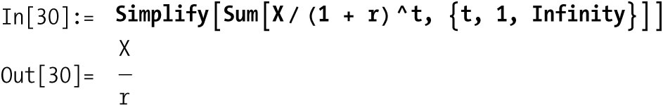
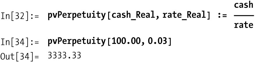
An annuity is a set of fixed cash flows
X that repeat for a specified
number of periods T.
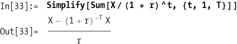
Hence...

Closely related to present value is the internal rate
of return, the rate that would make the present value equal
to zero. You can use FindRoot to
calculate the internal rate of return for a set of cash flows. Here we
tell FindRoot to begin searching
for a solution at irr of 0.0.

In finance, it is more common to deal with continuously compounding interest than the discrete compounding formulas discussed. The present value in terms of continuously compounding interest is
In[39]:= pvCC[cashFlows_List, times_List, rate_Real] :=
          Module[{N = Length[cashFlows]},
           Sum[cashFlows[[i]] / E^ (rate*times[[i]]),
           {i, 1, N}]]
In[40]:= pvCC[{-1000.0, 100.0, 300.0, 600.0, 600.0}, {0, 1, 2, 3, 4}, 0.05]
Out[40]= 374.237
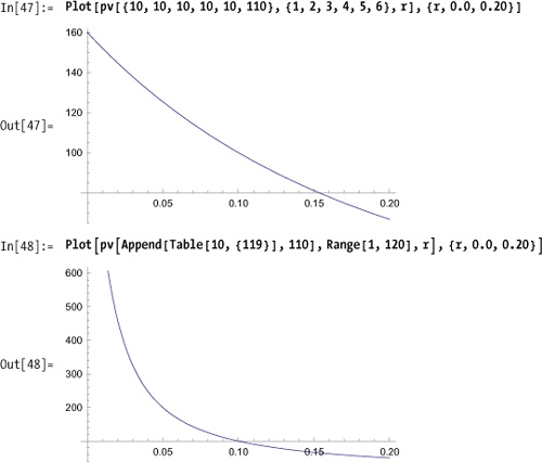
You want to determine the fair value of a bond and analyze its performance under varying market conditions.
Before you can analyze a bond, you need to know how to compute its price and yield to maturity. The price of a fixed-rate bond is equivalent to the present value of the bond’s coupon payments. For example, if a three-year bond has a face value of $100 and makes yearly payments of 10% and the present interest rate is 8%, then the fair bond price should be
In[41]:= pv[{10, 10, 110}, {1, 2, 3}, 0.08]
Out[41]= 105.154
The price only captures one aspect of a bond. You may also want to know the effective interest rate of the bond if it is held to maturity (yield to maturity). This is the same as the internal rate of return calculation of 12.1 Computing Common Statistical Metrics of Numerical and Symbolic Data. The first cash flow is the bond’s price, then the two coupon payments, and the final is coupon plus face value.

It is no accident that the yield to maturity is equal (modulo rounding errors) to the current interest rate. This is a sign that the bond is priced correctly.
Investors in bonds want to understand a bond’s sensitivity to changes in current interest rates. The price of an asset with long-term cash flows has more interest-rate sensitivity than an asset with cash flows in the near future. The duration is a weighted average maturity of a bond.
In[43]:= duration[cashFlows_List, times_List, rate_Real] :=
          Module[{T = Length[cashFlows], D, B},
          {D, B} = Sum[{(times [[t]] * cashFlows [[t]]) / (1 + rate) ^times[[t]],
               cashFlows[[t]] / (1 + rate) ^times[[t]]}, {t, 1, T}]; D/B]

In[44]:= duration[{10, 10, 110}, {1, 2, 3}, 0.08]
Out[44]= 2.74236

In[45]:= convexity[cashFlows_List, times_List, rate_Real] :=
          Module[{T = Length[cashFlows], B},
          B = pv[cashFlows, times, rate]; (1 / B)* (1/ (1 + rate)^2) *
           Sum[(times [[t]] + times [[t]] ^2) *
               (cashFlows [[t]] / (1 + rate) ^times [[t]]), {t, 1, T}]]

In[46]:= convexity[{10, 10, 110}, {1, 2, 3}, 0.08]
Out[46]= 9.11374
You want to build a yield curve from underlying spot rates and then model changes in the curve so you can model the return of a portfolio of rate-sensitive securities.
If you are only interested in changes in the yield curve at a
particular maturity, you can use published yields for various
maturities and use interpolation. For example, here is some interest
rate data taken from Bloomberg in late June 2009. The pairs are
{days, rate}.

Interpolation is all well and good, but if you want to understand the dynamics of the curve, you need a model. The Nelson-Siegel function is a popular parametric model of the yield curve.

Here I use the fitted curve to initialize a Manipulate. You can then play with the
parameters to get a feel for their effect.

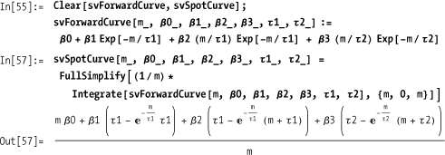
An extension of the Nelson-Siegel model is the Svensson model, which addresses problems with convexity, inaccuracies introduced for large changes in yield due to the nonlinear relationship between prices and yields. The capital gain induced by a decline in the yield is larger than the capital loss induced by an equal-sized increase in the yield.
Given the Svensson model for the forward curve, you can use Mathematica’s symbolic integration capabilities to find the zero coupon (or spot) model.
The solution demonstrates a so-called parametric method (i.e., a method based on parameters that have real-world meaning). There are also nonparametric methods that are in use where curves are fit using polynomials and tension splines. See the following references.
This recipe is based on Parsimonious Modeling of Yield Curves by Charles R. Nelson and Andrew F. Siegel (Journal of Business, Vol. 60, No. 4 [Oct. 1987]: 473-489), which can be found online at http://bit.ly/1mQ3mq .
A library of Mathematica code for working with the term structure of interest rates can be found on Mark Fisher’s website at http://bit.ly/3hW4KC , with documentation at http://bit.ly/1ormSc .
A more thorough investigation of yield curve models can be found in this notebook at the Wolfram Library Archives, http://bit.ly/17OU4U , which was developed by Jan Hurt of the Charles University of Prague.
We give the solution to the Black-Scholes formula here
without derivation. There are many excellent resources listed in the
See Also section for readers interested in
the theory underlying this solution. The helper functions dl and d2
have become fairly standard within the literature, so I use them here
despite my personal aversion to short, cryptic names. The expression
involving the dl term in the
pricing functions is related to the value of acquiring the stock; the
expression involving the d2 term
relates to the value of exercising the option on expiration.
In[58]:= Clear[d1, d2, priceEuroCall, priceEuroPut]These helper functions are used by both priceEuroCall and priceEuroPut.
In[59]:= d1[price_Real, strike_Real, volatility_Real, maturityT_Real, rate_Real] :=
            (Log[price/ strike] + (rate + volatility^2./2.) *maturityT) /
             (volatility * Sqrt[maturityT]);
         d2[price_Real, strike_Real, volatility_Real, maturityT_Real, rate_Real] :=
           d1[price, strike, volatility, maturityT, rate] -
            volatility * Sqrt[maturityT];
         cumNormDist[x_?NumberQ] := CDF[NormalDistribution[], x];
Given the price of a stock, the strike price of the option, the volatility, time to option maturity in fractions of a year, and the risk-free interest rate, compute the value of a call or put option.
In[62]:= priceEuroCall[price_Real, strike_Real,
           volatility_Real, maturityT_Real, rate_Real] :=
          price*cumNormDist[d1[price, strike, volatility, maturityT, rate]] -
           strike* Exp[-rate* maturityT] *
            cumNormDist[d2[price, strike, volatility, maturityT, rate]]
The fact that a put can be priced in terms of a call is called put-call parity.
In[63]:= priceEuroPut[price_Real, strike_Real, volatility_Real, maturityT_Real,
           rate_Real] := priceEuroCall [price, strike, volatility, maturityT, rate] +
           strike * Exp[-rate * maturityT] - price
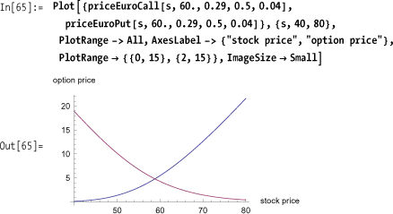
Here we compute the value of a call option with strike $60 and 1/2 year to maturity, with the underlying stock trading at $70, with a volatility of 0.29, and a risk-free rate of 4%. The volatility is usually measured as the standard deviation of the stock price.
In[64]:= priceEuroCall[70., 60., 0.29, 0.5, 0.04]
Out[64]= 12.6323
Here we show the opposing relationship between a call and a put with equal attributes by plotting their values against the price of the underlying stock. A call increases in value with the stock price, whereas a put decreases in value.
Although the ability to price an option is vital to successful trading, it is equally vital to measure the sensitivity of an option (or any other derivative security) to changes in the economic environment. These measures are based on mathematical derivatives of the pricing function. These measures are collectively known as the Greeks because each is associated with a Greek letter.
In[66]:= Clear[deltaEuroCall, deltaEuroPut,
          gammaEuroCall, gammaEuroPut, thetaEuroCall, thetaEuroPut,
          rhoEuroCall, rhoEuroPut, vegaEuroCall, vegaEuroPut]
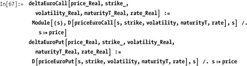
Delta is a measure of the sensitivity of an option to changes in the stock price. It is computed as the first derivative of the pricing function with respect to the underlying stock price.
Gamma is a measure of the sensitivity of the delta to changes in the stock price. It is computed as the second derivative of the pricing function with respect to the underlying stock price.

Theta is a measure of the sensitivity of the option price to time. It is computed as the first derivative of the pricing function with respect to the time to expiration (maturity).

Rho is a measure of the sensitivity of the option price to changes in the risk-free rate. It is computed as the first derivative of the pricing function with respect to the interest rate.

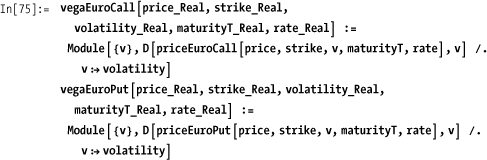
Vega (also known as kappa) is a measure of the sensitivity of the option price to changes in the volatility. It is computed as the first derivative of the pricing function with respect to the volatility.
Here we compute delta of a call with strike $60 with 6 months left to maturity when the stock is trading at $40. This shows that the option will change value by roughly 3.7 cents for a dollar move. We can confirm this using the pricing function.
In[77]:= deltaEuroCall[40.00, 60., 0.29, 0.5, 0.04]
Out[77]= 0.0377654
This is in basic agreement with the difference between the value of the option at a stock price of $40.50 and $39.50 (we choose a dollar spread that places the delta stock price at the center).
In[78]:= priceEuroCall[40.50, 60., 0.29, 0.5, 0.04] -
          priceEuroCall[39.50, 60., 0.29, 0.5, 0.04]
Out[78]= 0.0378454
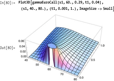
You can get an intuitive feel for the behavior of options by creating a 3D plot of each Greek with respect to stock price and time.
Note how delta increases sharply as the stock price approaches the strike and how this sensitivity is stronger near expiration (t = 0).

The sensitivity of the delta to shrinking time to maturity and strike price is reinforced by the plot of the gamma, which is the second derivative of the price, or the first derivative of the delta.
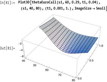
The plot of theta shows that the value of an option will decay more rapidly with adverse moves of the underlying stock when there is a short time to expiration compared to when there are longer times.

Note how sensitivity to volatility increases near the strike price and with increasing time. This follows from the fact that high volatility has more impact over longer time periods and for options that are in the money (because of the larger delta and gamma of in-the-money options).

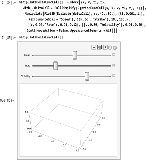
The interactive capabilities of Mathematica 6 provide an
excellent platform for getting the feel of the behavior of the Greeks.
However, for sake of responsiveness, it is a good idea to evaluate the
derivative outside the Manipulate.
You can use With to evaluate the
derivative before the call to Manipulate and FullSimplify to make sure it is in simplest
form.
Modeling Financial Derivatives with Mathematica (Cambridge University Press) by William Shaw is an excellent resource for the quant interested in modeling vanilla and more exotic flavors (such as Asian options) in Mathematica. It concentrates on analytical solutions rather than solutions based on numerical methods.
Black-Scholes and Beyond: Option Pricing Models by Neil A. Chris (McGraw-Hill) covers the basics of modern option pricing. Wikipedia also provides basic information on the Black-Scholes model: http://bit.ly/c8IrYX .
Use FindRoot to solve for the
volatility.
In[86]:= impliedVolEuroCall[price_, strike_, maturityT_, rate_, optionsPrice_] :=
          volatility /.
           FindRoot[priceEuroCall[price, strike, volatility, maturityT, rate] ==
             optionsPrice, {volatility, 0.2}]

In[87]:= impliedVolEuroPut[price_, strike_, maturityT_, rate_, optionsPrice_] :=
          volatility /.
           FindRoot [priceEuroPut [price, strike, volatility, maturityT, rate] ==
             optionsPrice, {volatility, 0.2}]

In[88]:= impliedVolEuroCall[58.00, 60., 0.5, 0.04, 3.8]
Out[88]= 0.254867
Implied volatility is the volatility that is implied by the market price of the option given the pricing model. The idea is that the market will find the fair price for the option, and from that, you can back out the volatility of the underlying security that the market is pricing in. This is in contrast to historical volatility, which is a direct measure of the movement of the underlying’s price over recent history.
In the solution, FindRoot
searches for a numerical root of the pricing function that will yield
the observed price, given the other option parameters.
You want to compute numerical solutions to partial
differential equations (PDEs), such as the Black-Scholes PDE. NDSolve can sometimes take too much time or
lose accuracy near critical values. You would like to speed up
NDSolve without loss of accuracy
where it matters.
This recipe was motivated by work done by Andreas Lauschke and used with permission. Refer to the See Also section for more information.
To illustrate the problem, I use the PDE for a European put on a dividend-paying security. For the interest and dividend, I use fixed rate plus time-varying rate that is strictly increasing. For volatility, I use a volatility smile, which reflects the observation that volatility is higher for in- and out-of-the-money options and lower for at-the-money options. In the PDE, x represents the price of the underlying and t is time.

You can adjust different aspects of this model to suit your
needs. The main point here is to consider the performance of NDSolve using different options.

It took just over eight seconds to solve this PDE
numerically. However, you can do better using an adaptive grid method
where you instruct NDSolve to
sample more points around the strike price while being looser away
from the strike. Here I define a function for the adaptive grid but
defer explanation until the discussion.

You can see the speedup is quite substantial.
In[102]:= timePut1 / timePut2
Out[102]= 23.3068You can see that the result of pricing the option appears the same for both versions.

And, indeed, you can see that the max difference in both approaches is negligible.
In[104]:= Max@
           Flatten@Abs[Table [(u [x, t] /.First@put1), {x, 40, 60}, {t, 0, 1, 0.01}] -
              Table[(u[x, t] /. First@put2), {x, 40, 60}, {t, 0, 1, 0.01}]]
Out[104]= 0.0000251351
A few words about the function makeAdaptiveGrid are in order. The
motivation for this function can be seen considering the plot of
x^3.

The slope about the origin is small compared to the slope at the
extremes. This is perfect for our application because it means that
simply shifting the origin to the strike will give a function that
generates a dense grid around the strike and a looser one at the wings
of the option (away from the strike). The two optional parameters of
makeAdaptiveGrid control the number
of grid points (size) generated and
the extent of the density around the slope (deg).

In the NDSolve
options, I use MethodOfLines, which
is a very efficient way to numerically solve a PDE provided it is an
initial value problem. In particular, the solution uses the suboption
"SpatialDiscretization", which
itself allows the coordinates to be passed in. Here the expression
N@Union[makeAdaptiveGrid[strike], Range[2
        strike, 5 strike, 2]]
simply tacks on some coarsely spaced
points far from the strike so we can ensure the solution is valid for
a reasonably liberal range of prices on the high end. Refer to the
references in the following See Also
section for more details about MethodOfLines, which is quite feature rich
and worth learning if you plan to use NDSolve.
This recipe was motivated by the notebook penalty.nb developed by Andreas Lauschke.
The original notebook is available in the downloads section of this
book’s website: http://bit.ly/xIgx7
. Also see Lauschke’s site at http://bit.ly/1Zhdfv for useful Mathematica
and web Mathematica samples, products, and services.
NDSolve was introduced in
13.9 Modeling a Vibrating String.
The MethodOfLines can be
found in tutorial/NDSolvePDE in the Mathematica
documentation.
You want to use the finite difference method (FDM) to compute solutions to the Black-Scholes formula in an efficient manner.
This solution was developed by Thomas Weber and rearranged to conform to the format of this book. Refer to the See Also section for references to the original notebook.
In this solution we will price a European call option with the following attributes:
In[108]:=  strike = X = 100.; (*strike price at maturity of the option*)
           sigma = σ = 0.2;   (*volatility of the prices of the underlying*)
           tau = τ = 1.0;     (*time to maturity of the option*)
           rate = r = 0.05 ;  (*riskless interest rate*)
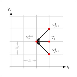
The presented calculation scheme is a version of the explicit finite difference method (FDM). While applying this calculation scheme, the new values for the derivative Vj,i–1 are stepwise calculated from Vj+1,i, V j,i , and Vj–1,i. The concepts are elaborated in the Discussion section.
In this solution, the number of grid points for the discrete
prices of the stock n can freely be
chosen within a specific range. Increasing the number of time steps
improves the accuracy but also increases the overall calculation time.
For a first demonstration, the number of discrete stock prices is set
to 20.
In[112]:= n = 20;The grid points for the stock price should be placed in a range
not too tight around the current stock price. In this example, the
range is chosen from zero up to twice the strike price. From the
chosen region results the step size ΔS for the discretization of the
stock prices range. One way to generate the list of grid points is to
use NestList. #+ΔS& within NestList is a generic function defined for
local use.
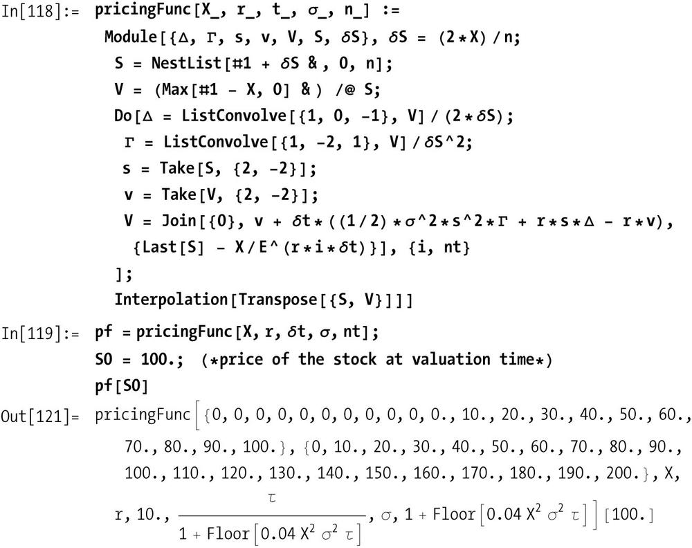
On the list of discrete stock prices, the exercise function of the option can be applied. The resulting list provides the starting or initial values for the numerical method.
In[113]:= δS = (2 * X) / n;
          S = NestList[#1 + δS &, 0, n];
          V = (Max[#1 - X, 0] &) / @ S;
The necessary number of time steps for the explicit FDM to converge depends on the step size for the discretization of the stock price, the volatility, and the strike price. The number of time steps can be calculated as follows (for more information, see the Wilmott reference in the See Also section):
In[116]:= nt = Floor[τ /(δS / (2*×*σ] ^2 + 1;Then the size of the time steps are
In pricingFunc, two terms
r and Δ (see the Discussion section) are the speed-critical
computations since they are inside the Do loop. The Mathematica function ListConvolve is used because it is a very
fast way to compute finite differences. After the Do loop is finished, V contains a list of option values. Each
option value corresponds to a discrete stock price on the grid.
Interpolation on these numbers
produces an interpolating function for the option price given current
price of the underlying
S0.
The PDE from the Black-Scholes formula for a derivative V on the security S is given as:
In[122]:= Clear[S, δS, t, δt, σ, r, V];
          pde = -D[V[S, t], t] ==
             (1/2) *σ^2 * S^2 * D[V[S, t], S, S] + r * S * D[V[S, t], S] - r * V [S, t];
Numerical approximation for the partial derivative follows, for example from the Taylor series. The partial derivatives in the equation are replaced through the appropriate Taylor series.
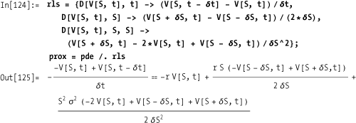
In the next step, the notation is changed to make it more consistent with a grid scheme.
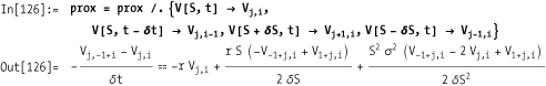
To better illustrate the structure of the equation, more notational adjustments are made. The new structure will later help to simplify the calculations.

Solving the last expression for Vj,i and simplifying leads to

The presented calculation scheme is a version of the explicit FDM. While applying this calculation scheme, the new values for the derivative Vj,i–1 are stepwise calculated from V j+1,i, V j,i , and V j–1,i . Figure 14-1 illustrates this approach.
An efficient Mathematica function for the calculation of
the differences needed in Δ and
r is available through ListConvolve. To demonstrate this, ListConvolve is applied to a list of
symbols.
In[130]:= Clear[V, δS];
          v = Table[Vj, {j,6}]
Out[131]= {V1, V2, V3, V4, V5, V6}
ListConvolve used for Δ
results in the following expression.
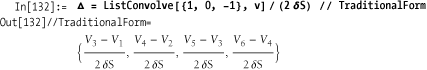
The first list in ListConvolve, the kernel {1, 0, 1}, is applied piecewise to the
second list, multiplies the elements of the second list, and adds them
up according to the values given in the kernel. This operation runs
internally in Mathematica and is much faster than any loop written in
Mathematica code.
The approach used for Δ can also be applied for the calculation
of r. ListConvolve can replace
loops that are common to the explicit approximation of PDEs.

Derivatives: The Theory and Practice of Financial Engineering (Wiley) by P. Wilmott contains the technical background underlying this recipe.
This recipes was derived from work done by Thomas Weber of Weber & Partner. The original notebook and other interesting financial applications in Mathematica can be found at http://bit.ly/bR0bF .
The method used in this recipe is based on the explicit FDM. There are also implicit methods. See Wikipedia for a general explanation of the difference and the tradeoffs ( http://bit.ly/tr3IN ).
You need a very fast pricer for American options. You want to make sure the implementation can be compiled for fastest possible execution without any calls to non-compiled code.
This solution was contributed by Andreas Lauschke. See 14.8 Speeding Up NDSolve When Solving Black-Scholes and Other PDEs for more information.
Mathematica has a built-in compiler that creates optimized code
for a Mathematica-specific virtual machine. Compile is discussed fully in 18.5 Compiling Functions to Improve Performance. Here we simply
show an application that creates a pricer for American options using
trinomial scheme (see discussion).
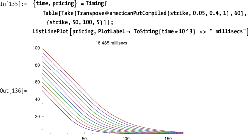
In[134]:= americanPutCompiled = Compile[{kk, r, sigma, tt},
             With[{a = 5, nn = 100, mm = 20, tt0 = sigma^2 tt/2, k = 2 r / sigma^2},
              Module[{alpha, h = 2 a / nn, s = tt0 / mm, x, ss, tmax, f, pp0, u, z},
               alpha = s/h^2;
               x = Range[-a, a, h];
               ss = kk Exp@x;
               tmax = MapThread[Max, {Table[0, {nn + 1}], 1 - Exp@x}];
               f =
                Exp[1/2 (k - 1) x + 1/4 (k + 1) ^2 (# - 1) s] tmax& /@ Range [mm + 1];
               pp0 = Max [0, kk - #] & /@ ss;
               u = Exp[1/2 (k - 1) x] pp0 / kk;
               Do[z =alpha (Take[u, {3, nn +1}] + Take[u, {1, nn -1}]) -
                  (2 alpha -1) Take[u, {2, nn}];
                z = Append[Prepend[z, alpha u[[2]] - (2 alpha - 1) u[[1]] +
                    alpha/kk Exp[1/2 (k -1) a+1/4 (k +1) ^ 2 (j -1) s]], 0];
                u = MapThread[Max, {z, f[[j]]}];, {j, mm}];
                {ss, kk Exp[-1/4 (k +1) ^ 2 tt0] Exp[-1/2 (k -1) ×] u}]]];
You can see that 10 runs of the pricer over various strike prices execute in 32 milliseconds.
The function americanPutCompiled returns a packed array
of two lists: the first is a list of nodes in the spatial (stock
price) direction, and the second is a list of American option prices
at these nodes. The two lists can now be interpolated with
Mathematica’s Interpolation
function to obtain intermediate values.
The function americanPutCompiled is fully compiled, as
can be seen by inspecting americanPutCompiled[[4]] and noting that all
list elements are numeric.
In[137]:= DeleteCases[Flatten[americanPutCompiled[[4]]],_?NumericQ]
Out[137]= {}
The algorithm implements a method to price American options
based on the linear complementarity formulation of the free boundary
value problem. The numbers a, nn,
TO, and mm (and,
correspondingly, s and h) are parameters that define the grid to be
used. a and nn determine the grid along the space (stock
price) axis, and TO and mm determine the grid along the time axis.
For explicit methods, it is crucial to keep the spatial and temporal
spacing in certain limits, otherwise local blow-up will occur. For a
100% explicit method, it is necessary that alpha=s/h^2<=1/2. That means that if the
spatial step size h is reduced by a
factor of 10, the time step size s
has to be reduced by a factor of 100. This is not due to reasons of
precision, but due to reasons of stability. If, for example, mm is lowered to 15, alpha is no longer <=1/2, and the instability becomes quite
visible. For numbers like 5 or 10 for mm, the method wreaks havoc. Traditional American option pricing methods use
binomial trees and exhibit this problem with what is called
oscillations. (All tree methods are necessarily
100% explicit.) It’s the same stability problem that is inherent to
all explicit methods.
What makes this rectangular grid method so powerful is the fact that although it is faster than most tree-based implementations, it computes the option prices for the whole interval, not just for one particular price of the underlying, which is a limitation all tree-based methods possess.
18.5 Compiling Functions to Improve Performance explains the mechanics of compiled functions and the performance implications of functions that don’t fully compile.
See Ansgar Jüngel, "Modellierung und Numerik von Finanzderivaten," Vorlesungsmanuskript 2002, Johannes-Gutenberg Universität Mainz.
You want to understand the worst expected loss of a portfolio of securities. This is referred to as Value-at-Risk or VaR. Specifically, you want to use Monte Carlo methods because these allow you to trade accuracy for speed by varying the number of samples.
Note
Since the financial disaster that began in 2007, the notion of Value-at-Risk has become quite controversial. Some, like Nassim Taleb, have called it an intellectual fraud, while others have called it an invaluable tool, if used properly. I include this recipe as an illustration of the math behind one particular implementation of VaR and without judgment as to its effectiveness. Please refer to the link in the See Also section for a thorough discussion of the efficacy of VaR in practice.
In its simplest form, VaR is a measure of the worst expected loss under normal market conditions over some time interval, usually days or weeks. The simplest (and highly artificial) illustration of VaR concerns a portfolio consisting of a single security. Let’s assume it is worth $10 million, the average return is 0.085, and the standard deviation is 0.26. The distribution of the portfolio’s value is

From this we can compute the probability of a loss of 25% using the CDF.
In[139]:= With[{portfolio = 10000000, return = 0.085, stddev = 0.26, loss = 0.25},
           CDF[NormalDistribution[portfolio * (1.0 + return), portfolio *stddev ],
            portfolio (1 - loss)]]
Out[139]= 0.0987927
VaR is computed in terms of worst expected loss in dollars at a certain probability level, say 1%.
In[140]:= valueAtRisk[startingValue_, meanReturn_, var_, level_] :=
           Module[{expected = startingValue* (1 + meanReturn)},
            startingValue -
             Quantile[NormalDistribution[expected, startingValue * var], level]]

In[141]:= With[{portfolio = 10000000,
            meadReturn = 0.085, stddev = 0.26, loss = 0.25},
           valueAtRisk[portfolio, meadReturn, stddev, 0.01]]
Out[141]= 5.1985×10⁶
Thus the VaR at 1% is about 5.2 million.
The solution merely shows the statistical ideas behind VaR. In real-life scenarios, portfolios are more complexly structured, and you need to measure and account for correlations in the movements of these assets’ values. The rest of this discussion deals with these issues.
The first issue to address is that prices don’t typically follow
a NormalDistribution but rather a
LogNormal one. Second, portfolio
managers and traders are typically interested in VaR over much shorter
time periods than one year. So a more useful function is
In[142]:= Clear[valueAtRisk]
          valueAtRisk[ startingValue_, mean_,
            var_, level_, days_, tradingDays_: 365] :=
               Module[{T = days / tradingDays},
            startingValue - Exp[Quantile[NormalDistribution[
                Log@startingValue + (mean - var^2 / 2) * T, var * T], level]]
           ]
Here we compute the VaR assuming 250 trading days.
In[144]:= With[{portfolio = 10000000,
            return = 0.085, stddev = 0.26, loss = 0.25, days = 1},
           valueAtRisk[portfolio, return, stddev, 0.01, days, 250]]
Out[144]= 22121.5
An extensive discussion of VaR in light of the financial crisis of 2007-2009 (and counting) can be found in this excellent New York Times article by Joe Nocera: http://bit.ly/2SgV68 .
You are using a tree-based approach to pricing (such as the Hull-White trees) and you want to visualize these trees using Mathematica’s graphics abilities. Such visualizations are often useful for pedagogical or diagnostic purposes.
In this recipe, I am only concerned with using Mathematica for visualizing Hull-White trees. See the See Also section for the theory and Mathematica implementation of the same for pricing purposes.
The usual way to implement tree valuation methods is to state results in two or more new states, thereby modeling the diffusion of the stochastic process. The idea of Hull-White to model mean reverting processes is to add boundary conditions to this tree structure. The boundary conditions are valid for a given maximum state.
The graphical building blocks of the tree can then be defined as
follows. The variable nmax is
global. There are three primitive elements: a nonboundary element, an
upper-boundary element, and a lower-boundary element. The function
path returns a triple that defines
the terminal points of the path.
In[145]:= path[j_] :=j + {1, 0, -1}
          path[j_ /; j == nmax] := j - {0, 1, 2}
          path[j_ /; j == -nmax] := j + {0, 1, 2}
The function grpath then
constructs the graphical representation in terms of Line elements emanating from a starting
point.
In[148]:= grpath[pt: {i_, j_}] := Line[{pt, {i + 1, #}}] & /@ path[j]Here then are the three primitive components used to build the tree.
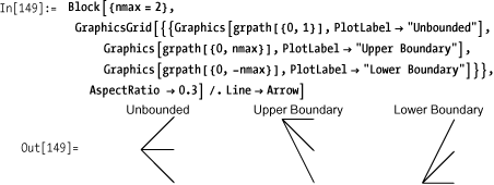
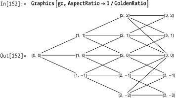
Given these primitives, it’s a straightforward process to generate a tree with a particular boundary and depth.

The solution is really just a skeleton to illustrate the general technique. For purposes of visualization, we need trees with labels that suggest the underlying semantics of Hull-White. A particularly nice way to proceed is to augment the tree with node labels that are purely coordinates. This is just a matter of adding text elements to the solution version. The resulting gr becomes a template, and you can leverage Mathematica’s pattern-directed replacement to assign meaningful labels to the nodes.

The process you want to visualize is a single-factor interest rate model described by the following formula:
dr = (θ(t) - a rt) dt + σ dz.Here r is the short-term
rate, and a and σ are constants.
In[153]:= a = 0.1;
          σ = 0.01;
          Δt = 1;
          Δr = σ*Sqrt[3 * Δt];
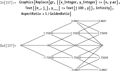
Using the template gr,
replace the nodes with the rate deltas using the node coordinates in
the computation of the labels. Here you use depth Infinity with Replace so you need not worry about the
actual depth of the graphics elements.
This recipe contains content originally developed by Thomas Weber of Weber & Partner ( http://bit.ly/3Dz1wg ) and is used with permission. A complete notebook showing both the theory and visualization is available at this cookbook’s website: http://mathematicacookbook.com/downloads/index.dot .