You have an executable program that you would like to launch from Mathematica.

Use Run to execute command line programs. Run returns the exit code of the program. Results can be read in from a file written by the program. Here is an example that will work on the Windows operating system. This is only to illustrate the technique. Mathematica is perfectly capable of telling you the date itself.

You can also read the output of external programs by using the escape character ! and the function ReadList. This example uses the GNU program wget to retrieve a web page and extract the unique URLs. Note that this example assumes you have wget installed on your system and that it is in the path the Operating System (OS) uses to find programs.

webpage = ReadList["!wget -0 - http://www.wolfram.com", String];
Union[Flatten[StringCases[webpage, RegularExpression[
    "https?://([-w.]+)+(:d+)?(/([w/_.]*(?S+)?)?)?"]]]]
{http://blog.wolfram.com/,
 http://demonstrations.wolfram.com/, http://functions.wolfram.com/,
 http://integrals.wolfram.com/index.jsp, http://library.wolfram.com/,
 http://mathworld.wolfram.com/, http://partnerships.wolfram.com/,
 http://reference.wolfram.com/alphaindex/,
 http://reference.wolfram.com/mathematica/guide/Mathematica.html,
 http://register.wolfram.com/, http://search.wolfram.com/,
 http://store.wolfram.com/, http://store.wolfram.com/catalog/,
 http://store.wolfram.com/view/app/mathematica/upgrade.upg,
 http://support.wolfram.com/, http://tones.wolfram.com/,
 http://www.mathematica-journal.com/issue/v10i3/,
 http://www.stephenwolfram.com/, http://www.w3.org/1999/xhtml,
 http://www.w3.org/TR/xhtml1/DTD/xhtml1,
 http://www.wolfram.com/services/education/seminars/,
 http://www.wolframscience.com/}

Additional details about running external programs can be found in the Mathematica tutorial /ExternalPrograms.

You want to launch a Windows-based program from the frontend and Run["Program"] does not work.

Use the Windows Start command in the Run so the program is launched indirectly.

Run["Start WinWord"]; (*starts MS Word*)

I ran across this problem while preparing a presentation in Mathematica for which I wanted to have a button that launched XMLSpy to show some XML. Without the use of Start, you need to specify the full path to the executable; Mathematica complains because it expects the command to be short-lived. Note that Start is a Windows command and not a Mathematica one.

The above problem could be solved using Method "Queued" as an option to Button, but using Start is much simpler.

You want to use the Mathematica kernel from a different computer than the one you are using to run the frontend.

Use the menu Evaluation, Kernel Configuration to create a configuration for a remote kernel. Select Add from the dialog. You will then be presented with the Kernel Properties dialog shown in Figure 17-1. It makes sense to give the kernel a meaningful name that will remind you what server it is connected to, but you can name it after your spouse or your dog if you like. Select the radio button Remote Machine and then enter the machine’s name, a login name, and the kernel program (which is often "math," but see the Discussion section). I like to check the option "Append name to In/Out prompts" to remind me I am working with a remote kernel, but this is a matter of taste. If you will mostly be working with this specific remote kernel, you can also check the automatic launch option.

Figure 17-1. Kernel Properties dialog

When you have the kernel configured, you can use Evaluation, Start Kernel to start it and Evaluation, Notebook Kernel to associate it with the current notebook.

If you have network access to a more powerful computer than the one you use daily and that computer has Mathematica installed, then you can reap a lot of benefit from using a remote kernel. For example, I like to work on my laptop because it gives me the flexibility to work anywhere in my house. However, my basement has my powerful Mac Pro, so I usually run my kernel there. This not only gives me access to a faster machine, but frees resources on the laptop that would otherwise be used by the local kernel.

There is a caveat to the solution. If the machine you are connected to is a Mac, there is no program called "math." You must instead give the full path to the program called MathKernel in the edit box for Kernel Program. The location will depend on where Mathematica was installed. For example, I installed Mathematica under /Applications/Wolfram, so I entered /Applications/Wolfram/Mathematica.app/Contents/MacOS/MathKernel.

If you have trouble connecting to the remote kernel you should take the following steps.

You want to call C functions from Mathematica.

Here I demonstrate the process of creating a C program with functions that can be invoked from Mathematica. This example uses Microsoft Visual C++ 2005. Refer to the See Also section for information on using other programming environments. The simplest way to interface Mathematica to C is to utilize the preprocessor mprep, which takes a template file describing one or more C functions, and generate the glue code needed to interface those functions to Mathematica. Here is an example of an mprep file describing three different functions.

:Begin:

:Function:      fExample1
:Pattern:       fExample1[x_Integer, y_Integer]
:Arguments:     {x, y}
:ArgumentTypes: {Integer, Integer}
:ReturnType:    Integer

:Function:      fExample2
:Pattern:       fExample2[x_List, y_List]
:Arguments:     {x, y}
:ArgumentTypes: {IntegerList, RealList}
:ReturnType:    Integer

:Function:      fExample3
:Pattern:       fExample3[aStr_String]
:Arguments:     {aStr}
:ArgumentTypes: {String}
:ReturnType:    String

:End:

The C source code corresponding to these definitions follows. Note that lists are passed as pointers to arrays and that an extra integer parameter is needed for each such list to receive the length of the array. In this listing, you will also find the definition of WinMain that is required for Windows executables built with Microsoft Visual Studio. The body of WinMain is standard boilerplate that you can copy into your own project. The implementation of the functions themselves is really not important in this code as its main purpose is to demonstrate the C interface mechanics.

//functions.h

extern "C"
{
int fExample1(int x, int y);
double fExample2(int * x, long xLen, double* y, long yLen);
char * fExample3(char * aStr);
}
//functions.cpp

#include "functions.h"
#include <mathlink.h>
#include <stdio.h>
#include <ctype.h>


int fExample1(int x, int y)
{
    return (x >> y) + 1;
}

double fExample2(int * x, int xLen, double* y, int yLen)
{
    double result = 0.0;
    int i = 0;
    for (; i<xLen && i<yLen; ++i)
    {
        result += x[i] * y[i] ;
    }
    for (;i < yLen; ++i)
    {
        result += y[i];
    }
    return result ;
}

char * fExample3(char * aStr)
{
     for(char *p=aStr;*p;++p)
     {
         *p = toupper(*p) ;
     }
     return aStr ;
}


int PASCAL WinMain( HINSTANCE hinstCurrent, HINSTANCE hinstPrevious,
LPSTR lpszCmdLine, int nCmdShow)
{
    char   buff[512];
    char FAR * buff_start = buff;
    char FAR * argv[32];
    char FAR * FAR * argv_end = argv + 32;
    hinstPrevious = hinstPrevious; /*suppress warning*/

    if( !MLInitializeIcon( hinstCurrent, nCmdShow)) return 1;
    MLScanString( argv, &argv_end, &lpszCmdLine, &buff_start);
    return MLMain( (int)(argv_end - argv), argv);
}

Once you have a MathLink program compiled to an executable, you can install it using Install. By default, Install will look in the current directory for the executable; either change the current directory or give Install the full path. Install returns a LinkObject, which can be used to get information about available functions and also to terminate the connection using Uninstall.

saveCurDir = Directory[] ;
SetDirectory[
  "oreilly\Mathematica Cookbook\codemathLinkExample\Debug"];
link =Install["mathLinkExample"];
SetDirectory[saveCurDir];

You can interrogate a link for the available functions.

LinkPatterns[link]
{fExample1[x_Integer, y_Integer],
 fExample2 [x_List, y_List], fExample3 [aStr_String]=

You call installed MathLink functions just like normal Mathematica functions.

fExample1[2000, 4]
126

fExample2 [{1, 2, 3}, {2.0, 4.0, 6.0, 8.0}]
36.

fExample3["Testing"]
TESTING

Uninstall[link]
mathLinkExample

Although the solution is fairly straightforward, there are numerous details that are specific to the OS and compilation environment (compiler and IDE or make system). The Mathematica documentation for MathLink contains detailed instructions for many common environments, and you should follow those directions carefully. It is highly recommended that you use either the example in the solution given or some of the simple examples that are installed with Mathematica to become familiar with the process before trying to interface your own C functions.

Often you will need to return objects more complex than integers and doubles from your C functions. If this is the case, you should specify a return type of Manual in the template file. Manual means that you will manually code the function to call the appropriate low-level MathLink C API functions needed to return the correct data to Mathematica.

//randomList.tm

#include <stdlib.h>
#include <mathlink.h>

:Begin:
:Function:      randomIntList
:Pattern:       randomIntList[n_Integer]
:Arguments:     {n}
:ArgumentTypes: {Integer}
:ReturnType:    Manual
:End:

extern "C" void randomIntList(int n)
{
    int* randData = new int [n] ;
    if (randData)
    {
        for(int i=0; i<n; ++i)
        {
            randData[i] = rand() ;
        }
        MLPutInteger32List(stdlink, randData , n);
        delete [] randData;
    }
    else
    {
       MLPutInteger32List(stdlink,0,0) ;
    }
}
saveCurDir = Directory[];
SetDirectory[
  "oreilly\Mathematica Cookbook\codemathLinkExample2\Debug"];
link2 = Install["mathLinkExample2"];
SetDirectory[saveCurDir];

LinkPatterns[link2]
{randomIntList[n_Integer]}

randomIntList[12]
{2287, 5306, 19 753, 3868, 19 313,
 1043, 29 879, 26846, 14625, 1380, 24555, 28439}

Uninstall[link2];

The example given illustrates the use of MLPutInteger32List to return an array of data as a list. The MathLink API contains many related functions for returning a variety of types, including integers, strings, lists, multidimensional arrays, and the like. This example also demonstrates that template files processed by mprep can mix source code with template directives.

Another common requirement is the need to execute initialization code once when you install the MathLink program. C-based initialization code can easily be added to the applications main() or WinMain(), but what about Mathematica code? A typical example is code that installs documentation for the installed functions. For this you use mprep’s :Evaluate: specifications. For an example of this see http://bit.ly/duSEnb.

Information on how to set up your C-built environment can be found at tutorial/MathLinkDeveloperGuide (Mac OSX), tutorial/MathLinkDeveloperGuide (Windows), and tutorial/MathLinkDeveloperGuide (Unix and Linux).

See ref/program/mprep in the Mathematica documentation.

You want to use Mathematica as a Java scripting language to prototype a Java application or leverage the functionality of Java classes.

Use the JLink` package and call InstallJava to make the Java runtime environment available to Mathematica. You can then create objects and call methods or load classes to access static methods just as if they were Mathematica functions.

Needs["JLink'"]
InstallJava[];
(*Create an instance of decimal format and
 call a method using prefix notation obj@method.*)
fmt = JavaNew["java.text.DecimalFormat", "#.0000"];
fmt@format[#] & /@ {1.0, 7.333, N [Pi], 1/3.}
{1.0000, 7.3330, 3.1416, .3333}

(*Load a class and call a static method using
 the full class name as if it were a package.*)
LoadJavaClass["java.lang.System"];
java'lang'SystenfcurrentTimeMillis[]
1 226 852 744 984

InstallJava takes options that control how the Java is loaded. CommandLine javapath allows you to specify the particular version of Java you want to load if you have several versions available. For example, CommandLine "c:\Program Files\Java \jre1.6.0_07\bin\java". ClassPath classpath is used to provide a classpath that is different from the default obtained from the CLASSPATH environment variable. If you require special Java Virtual Machine (JVM) options, use JVMArguments arguments .

When InstallJava is invoked several times during a Mathematica session, the subsequent invocations are ignored. However, sometimes you want to clear out the old JVM and start fresh. In that case, use ReinstallJava to exit and reload Java. This is especially useful if you are making changes to a Java Archive (JAR) that you are developing alongside the Mathematica notebook that uses it. ReinstallJava takes the same options as InstallJava.

The following example uses a genetic algorithm (GA) Java library called JGAP (see http://jgap.sourceforge.net/ ). GAs are in the class of evolutionary inspired algorithms typically used to tackle complex optimization problems. This example demonstrates an ideal blend of Mathematica and Java because it shows how easy it is to script a Java application and exploit the visualization features of Mathematica to investigate its behavior.

The example also illustrates the use of JavaBlock as a means of automatically cleaning up Java objects when they are no longer needed. It also shows how Java arrays of objects are replaced by Mathematica lists and how the translation is automated by JLink.

I implement the problem using a function called knapsack, which takes an optional fitness function. The reason for this will become apparent later. Most of the code within knapsack is straightforward use of JLink facilities interspersed with standard Mathematica code. The comments in the code point out what’s going on, and much of the detail is specific to the JGAP library and the knapsack problem. One thing that might trip you up in your own Java-interfacing projects is dealing with Java arrays of objects. There is no JLink function specifically designed to construct arrays. Instead, wherever you need to call a Java function that expects an array, simply pass it a Mathematica list of objects created with JavaNew and Jlink will translate. Mathematica’s Table is convenient for that purpose and it is how the following code creates an array of Gene objects. Likewise, when calling a Java function that returns an array, expect Mathematica to convert it to a list.

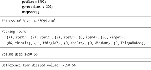
knapsack[fitnessFunc_ : None] :=
  (*Use a JavaBlock to release all Java objects when block completes.*)
  JavaBlock[
   Module[{conf, fitnessFunc2, sampleGenes, sampleChromosome, population,
     individuals, bestSolutionSoFar, packing, volumeFound, dummy},
    (*JGAP uses a configuration object to organize the
     genetic algorithm's parameters and objects.*)
    LoadJavaClass["org.jgap.Configuration"];
    Configuration'reset[];
    conf = JavaNew["org.jgap.impl.DefaultConfiguration"];
  (*We want to preserve the fittest individual.*)
  conf @ setPreservFittestlndividual[True];
      (*The fitness function is
       implemented as a class in the example code.*)
      fitnessFunc2 = If[fitnessFunc === None,
        JavaNew["examples.knapsack.KnapsackFitnessFunction", targetVolume],
        JavaNew["jgapMathematica.FitnessFunction", fitnessFunc]] ;
      conf@setFitnessFunction[fitnessFunc2];
      (*In the original Java code sampleGenes is a Java array of class
       Gene. However, in Mathematica you create lists of objects, and the
       JLink code will take care of translating to arrays when necessary.*)
      sampleGenes = Table[JavaNew["org.jgap.impl.IntegerGene",
         conf, 0, Ceiling [0.75 targetVolume/itemVolumes [[i]]]],
        {i, 1, Length[itemVolumes]}];

      sampleChromosome = JavaNew["org.jgap.Chromosome", conf, sampleGenes];
      conf @ setSampleChromosome[sampleChromosome];
         conf @ setPopulationSize[popSize];
         LoadJavaClass["org.jgap.Genotype"];
         population = org'jgap'Genotype'randomInitialGenotype[conf];
         (*Let's run the evolution for 200 generations and
          capture the fittest at each generation. *)
         {dummy, {saveFitnessValues }} = Reap [Do [population @ evolve[];
            Sow [population@getFittestChromosome[] @getFitnessValue []],
            {generations}]];
         bestSolutionSoFar = population@getFittestChromosome[];
      Print ["Fitness of Best:", bestSolutionSoFar@getFitnessValue []];
      (*Here we decode the best solution to get the qty of each item.*)
      packing =
          Table [{bestSolutionSoFar@getGene [i] @ getAllele[],
            itemNames[[i + 1]]}, {i, 0, bestSolutionSoFar@size[] - 1}];
      Print["Packing found: ", packing];
        volumeFound = Total[packing[[All, 1]] * itemVolumes];
      Print["Volume used ", volumeFound];
        Print["Difference from desired volume: ", targetVolume - volumeFound];
        ]
       ]

Using a fairly healthy population size and a large number of generations, we unfortunately get a fairly poor solution! This indicates a problem with the design of our GA. Let’s see how we can draw on Mathematica to help resolve this.

By plotting the logarithm of the fitness at each generation, we can see that the fitness landscape of this problem is extremely steep since we make a rapid transition from very low fitness to very high fitness. This suggests the fitness function provided with this JGAP sample might not be ideal. The poor quality of the solution is further indication of a poorly designed fitness function. The real lesson is that Mathematica is an ideal experimental playground for Java libraries because the full wealth of analytic and visual tools is at your disposal. In fact, I use Mathematica to help find a better fitness function, so read on.

If you want to experiment with Java libraries, it is ideal to be able to implement interfaces defined by those libraries directly in Mathematica. In fact, this can be done rather easily using ImplementJavaInterface. The following example uses Implement-JavaInterface to try an alternate fitness function for the knapsack problem. There is a caveat, however. ImplementJavaInterface will only work with true interfaces, not abstract classes. In JGAP, FitnessFunction is an abstract class, hence we can’t implement it using ImplementJavaInterface. The solution in cases like this is to create an adapter like the one in the following listing.

package jgapMathematica;

import org.jgap.IChromosome;

public class FitnessFunction extends org.jgap.FitnessFunction {

    private IMathematicFitness m_fitness;

    public FitnessFunction(IMathematicFitness fitness) {
        m_fitness = fitness ;

    }

    @Override
    protected double evaluate(final IChromosome chromosome) {
        return m_fitness.evaluate(chromosome);
        }

}

The above fitness function allows us to use the following interface within Mathematica code.

package jgapMathematica;

import org.jgap.IChromosome;

public interface IMathematicFitness {
    public double evaluate(final IChromosome chromosome) ;
}

Once this is done, we can write any fitness function we like in pure Mathematica code. This solution is general in that any abstract class you find in any Java library can be adapted in a similar manner. Below, we exploit the adapter to write a new fitness function for the knapsack problem. The function penalizes solutions that use more volume than specified, while giving increasing reward to solutions that use close to the available volume.

Keep in mind that implementing interface in Mathematica code is convenient but comes at a very high cost. In our case, it makes the GA run much slower and forces the use of a much smaller population size. This is especially true because the fitness function is called many times, and it must call back into Java, making it extremely costly. This is not a real issue because the goal here is experimentation. When a reasonable fitness function is found, it can be ported back to Java. You can use the same methodology when working with other Java libraries. Of course, if the interface you implement in Mathematica is called infrequently, the hassle of porting back to Java may seem unnecessary.

The J/Link tutorial is an excellent way to round out your knowledge of the Mathematica-to-Java interface. See JLink/tutorial/Overview.

Mathematica is bundled with notebooks illustrating different aspects of Mathematica-Java interaction (such as using the GUI features of Java Swing). These can be found in the Mathematica installation directory (evaluate $InstallationDirectory) under subdirectory SystemFiles/Links/JLink/Examples.

You want to use Mathematica as a .NET scripting language to prototype a .NET application or leverage Windows-specific functionality not directly available in Mathematica.

Use the NETI_ink~ package and InstallNET to initialize Mathematica’s .NET interface. You then can use functions like LoadNETAssembly to load custom .NET assemblies and NETNew to create instances of objects. Methods and properties of objects are accessed using Mathematica prefix notation object@property and object@method [args] .

As an example, you can use Mathematica 6’s dynamic functionality with a .NET timer to display a ticking clock.

Needs ["NETLink"']
InstallNET [];
timeOut = "Not Set";
timer = NETNew["System.Timers.Timer", 1000];
(*1 sec timer = 1000 msec*)
onTimedEvent[source_, eventArgs_] :=
  Module[{}, timeOut = eventArgs@SignalTime@ToString["G"]];
(*Use AddEventHandler to bind a Mathematica function to an event.*)
AddEventHandler [timer@Elapsed, onTimedEvent];
timer @ Enabled = True;
Dynamic[timeOut]
timeOut

timer@Enabled = False; (*Stop the timer*)

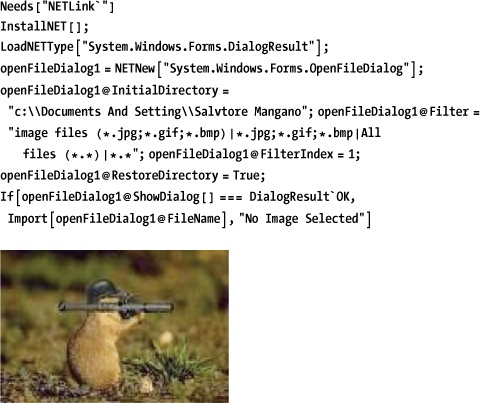
When you use NETNew, Mathematica implicitly loads the .NET type of the class you are creating. For some cases, you need to load the type explicitly. For example, many .NET components use Enums in their interface. To reference these in Mathematica code, you need to load them. In Mathematica, you use LoadNETType for this purpose. In the following example, you use LoadNETType to get the enumerations associated with dialog box results. This allows you to use the OpenFileDialog component to select a file. If you run this code, you may need to press Alt-Tab to switch to the dialog.

You also use LoadNETType to load a class that has a static method you want to call. Static methods are then accessible as normal Mathematica functions.

Needs["NETLink*"]
InstallNET[];
LoadNETType["System.Diagnostics.Stopwatch"];
System'Diagnostics'Stopwatch'GetTimestamp[]
5 674 487 004

The default value for the LoadNETType option StaticsVisible is False, but you can set it to True to avoid having to specify the full namespace path to invoke the function. You should use this feature with caution since it can lead to name conflicts.

An extensive tutorial on NETLink can be found in the Mathematica documentation at NETLink/tutorial/Overview.

You want to leverage the advanced Mathematica algorithms from within a .NET application.

Use the classes in the Wolfram.NETLink.dll from your .NET application. This recipe will use C#, but the Mathematica kernel is accessible from any .NET language. The simplest way to interact with Mathematica is through passing strings of Mathematica code using an instance of IKernelLink. You acquire an instance via MathLinkFactory.CreateKernelLink. IKernelLink has several methods for evaluating Mathematica code, but the function EvaluateToOutputForm is one of the most convenient.

using System;
using Wolfram.NETLink;

namespace TestNetLink1
{
     public class TestNetLink
     {

        public static void Main (String[] args)
        {

            //Launch the Mathematica Kernel
            IKernelLink ml = MathLinkFactory.CreateKernelLink ();
            //Discard the initial response kernel will send when launched.
            ml.WaitAndDiscardAnswer ();
            //Solve a differential equation and evaluate at the value 2
             string expr = "s = NDSolve[{y''[x]+Sin[y[x]] y[x] == 0,
                y[0] == i," +
                 "y'[0] == 0},y,{x, 0,30}]; y[2] /. s";
            string result = ml.EvaluateToOutputForm(expr, 0);
                Console.WriteLine ("Result = " + result);

            }
   }
}

Receiving numerical data back in string form is fine when you just want to display the result of a computation, but if you want to feed the results Mathematica returns into further computations, it is less than ideal. There are other ways to read the data returned by evaluation expressions, but these involve being cognizant of the types you expect back.

using System;
using Wolfram.NETLink;

namespace TestNetLink2
{

     public class TestNetLink2
     {

         public static void Main(String[] args)
         {

             //Launch the Mathematica Kernel
             IKernelLink ml = MathLinkFactory.CreateKernelLink();
             //Discard the initial response kernel will send when launched.
             ml.WaitAndDiscardAnswer();
             //Solve a differential equation and evaluate at the value 2.
             string expr = "s = NDSolve[{y''[x]+Sin[y[x]] y[x] == 0, y[0] ==
                1," +
                 "y'[0] == 0},y,{x, 0,30}]; y[2] /. s";
             //Evaluate expression. Notice this does not return anything.
             ml.Evaluate(expr);
             //Wait for results to be ready.
             ml.WaitForAnswer();
             //Read the result being sure to use the method that retrieves a

n

                appropriate
             //type. In this case, we expect a list of doubles but MathLink
                converts
             //these into arrays. Here you get the first element of the arra

y

                and can then
             //perform additional computations such as adding 10.
             double result = ml.GetDoubleArray()[0] + 10.0;
             Console.WriteLine("Result = " + result);
        }
    }
}

The IKernelLink interface has a variety of methods for retrieving typed results. These include GetBoolean, GetDouble, Getlnteger, GetString, GetDecimal, GetDouble-Array, and quite a few others. Refer to the NETLink documentation for the full set of methods.

In addition to IKernelLink, there is a very high-level interface to Mathematica implemented as a class called MathKernel that is ideal for creating a custom frontend to Mathematica. MathKernel derives from System.ComponentModel.Component and follows the conventions of .NET components. A nice example of using MathKernel can be found in the Mathematica installation directory ($InstallationDirectory) under SystemFiles/Links/NETLink/Examples/Part2/MathKernelApp.

You can find more information on interacting with the kernel from .NET languages at NETLink/tutorial/CallingMathematicaFromNET. There are examples there using both C# and Visual Basic.

You want to compute with data retrieved from an external database.

Note

The examples in 17.8 Querying a Database and 17.10 Introspection of Databases assume the existence of certain databases. If you don’t have access to a database system where you can set up these databases, the examples will obviously not work. If you have a database system or know how to install one, you can get files to initialize the database for these examples from the book’s website. Naturally, these examples are only for illustrating techniques that you can employ on real databases you wish to interface to Mathematica.

Mathematica supports several flavors of database connectivity, including ODBC, JDBC, MySQL, and HSQLDB (Hyper Structured Query Language Database).

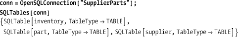
Here I open a connection to a SupplierParts database previously set up on my system and then query all rows of the part table. SQLSelect is the best way to retrieve all data from a single table. See the discussion for variations and alternatives.

Needs["DatabaseLink`"];
conn = OpenSQLConnection["SupplierParts"];
SQLSelect[conn, "part"]

{{pi, Nut, Red, 12., London}, {p2, Bolt, Green, 17., Paris},
 {p3, Screw, Blue, 17., Rome}, {p4, Screw, Red, 14., London},
 {p5, Cam, Blue, 12., Paris}, {p6, Cog, Red, 19., London}}

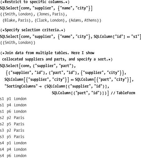
SQLSelect provides a stylized means to perform simple database queries without knowing SQL. Below are three increasingly complex queries you can do with SQLSelect.

Of course, the conventions used by SQLSelect create a very thin veneer over SQL, so if you plan to do quite a bit of database work, you will benefit from learning and using SQL directly via SQLExecute.

Nevertheless, using straight SQL can sometimes be a pain when you need to build the query from data stored in variables. SQLArgument, along with argument placeholders (e.g., `1`, `2`), is the recommended solution. You can use SQLArgument directly with values, but if you are parameterizing a query on column or table names, you must also use SQLColumn and SQLTable, respectively.

table = "supplier"; id = "s2"; col = "city";
SQLExecute[conn,
 "SELECT `1` FROM `2` WHERE id = `3`", {SQLArgument[SQLColumn[col]]
  SQLArgument[SQLTable[table]] , SQLArgument[id]}]
{{Paris}}

CloseSQLConnection[conn];

Detailed discussion of query commands can be found in DatabaseLink/tutorial/SelectingData in the Mathematica documentation.

You want to store results of computations to a database.

Use SQLInsert to add new records and SQLUpdate to modify existing records.

Needs["DatabaseLink`"];
conn = OpenSQLConnection ["MySQLTest"] ;

SQLInsert[conn,"data1", {"x1", "x2", "x3"},
  Table[{ i, Prime[i] , RandomReal[]} , { i, 1, 100}]] ;

SQLUpdate[conn, "data1", {"x1", "x2", "x3"},
 {0.0,1.0,2.0}, SQLColumn["data1.key"] == 4]
1

Use SQLDelete to remove records.

SQLDelete[conn, "data1", SQLColumn["data1.key"] == 10]
0

If you need to update multiple tables in an all-or-nothing manner and your database management system supports transactions, you should use SQLBeginTransaction and SQLCommitTransaction to bracket the updates. If an error occurs you can use SQLRollbackTransaction, which rolls back to the beginning of the transaction or to a named save point (which is set using SQLSetSavepoint).

Inserting, updating, and deleting are the most common operations for changing a database, but Mathematica also gives you the ability to create and drop tables.

SQLExecute[conn, "UPDATE data1 SET x1=0,x2=1,x3=2 WHERE data1.key=104"]
1

Detailed discussion of transactions can be found in DatabaseLink/tutorial/Transactions in the Mathematica documentation.

You want to query a database to find out what entities (tables, columns, etc.) are available.

Mathematica contains a variety of methods that return information about the data sources available, their tables, and the schema of those tables.

Needs["DatabaseLink`"]

The command DataSourceNames[] lists all data sources known to the Mathematica instance.

DataSourceNames[]
{demo, graphs, publisher, MySQLMeta, MySQLTest, SupplierParts}

Given a connection to one of these sources, list all the tables.

Given a connection, list all columns with their associated tables.

SQLColumnNames[conn] // TableForm
inventory sid
inventory pid
inventory qty
part      id
part      name
part      color
part      weight
part      city
supplier  id
supplier  name
supplier  status
supplier  city

You can also find out all the data types supported by your particular database.

SQLDataTypeNames[conn]
{BIT, BOOL, TINYINT, TINYINT UNSIGNED, BIGINT, BIGINT UNSIGNED,
 LONG VARBINARY, MEDIUMBLOB, LONGBLOB, BLOB, TINYBLOB, VARBINARY, BINARY,
 LONG VARCHAR, MEDIUMTEXT, LONGTEXT, TEXT, TINYTEXT, CHAR, NUMERIC,
 DECIMAL, INTEGER, INTEGER UNSIGNED, INT, INT UNSIGNED, MEDIUMINT,
 MEDIUMINT UNSIGNED, SMALLINT, SMALLINT UNSIGNED, FLOAT, DOUBLE,
 DOUBLE PRECISION, REAL, VARCHAR, ENUM, SET, DATE, TIME, DATETIME, TIMESTAMP}

CloseSQLConnection[conn];

The introspection commands demonstrated in the solution can take different arguments and options that restrict results or return additional information.

Needs["DatabaseLink`"]
conn = OpenSQLConnection["MySQLTest"];

For example, the SQLTables command can retrieve specific tables by name or using wildcards % (zero or more characters) and _ (any single character). By default, only tables are returned, but you can use the option TableType to list other tablelike entities, such as views.

If you are unsure what kinds of table types your database supports, you can list them with SQLTableTypeNames.

SQLTableTypeNames[conn]
{TABLE, VIEW, LOCAL TEMPORARY}

SQLColumnNames provides similar functionality. Here you can restrict columns to a particular table or columns in a table that match a pattern.

SQLColumnNames[conn]
{{data1, key}, {data1, x1}, {data1, x2}, {data1, x3},
 {data2, akey} , {data2, avalue} , {data1view100, key},
 {data1view100, x1}, {data1view100, x2}, {data1view100, x3}}

SQLColumnNames[conn, "data_"]
{{data1, key}, {data1, x1}, {data1, x2},
 {data1, x3}, {data2, akey}, {data2, avalue}}

SQLColumnNames[conn, {"data_", "x_"}]
{{data1, x1} , {data1, x2} , {data1, x3}}

Detailed discussion of descriptive commands can be found in DatabaseLink/tutorial/TableStructure and DatabaseLink/tutorial/ColumnStructure in the Mathematica documentation.