CHAPTER 12

Tools for Tree Searches: Branch-and-Bound and A* Algorithms

C. LEÓN, G. MIRANDA, and C. RODRÍGUEZ

Universidad de La Laguna, Spain

12.1 INTRODUCTION

Optimization problems appear in all aspects of our lives. In a combinatorial optimization problem, we have a collection of decisions to make, a set of rules defining how such decisions interact, and a way of comparing possible solutions quantitatively. Solutions are defined by a set of decisions. From all the feasible solutions, our goal is to select the best. For this purpose, many search algorithms have been proposed. These algorithms search among the set of possible solutions (search space), evaluating the candidates and choosing one as the final solution to the problem. Usually, the search space is explored following a tree data structure. The root node represents the initial state of the search, when no decision has yet been made. For every decision to be made, a node is expanded and a set of children nodes is created (one for each possible decision). We arrive at the leaf nodes when all the problem decisions have been taken. Such nodes represent a feasible solution. The tree structure can be generated explicitly or implicitly, but in any case, the tree can be explored in different orders: level by level (breadth-first search), reaching a leaf node first and backtracking (depth-first search), or at each step choosing the best node (best-first search). The first two proposals are brute-force searches, whereas the last is an informed search because it uses heuristic functions to apply knowledge about the problem to reduce the amount of time spent in the process.

Branch-and-bound (BnB) [1–4] is a general-purpose tree search algorithm to find an optimal solution to a given problem. The goal is to maximize (or minimize) a function f (x), where x belongs to a given feasible domain. To apply this algorithmic technique, it is required to have functions to compute lower and upper bounds and methods to divide the domain and generate smaller subproblems (branch). The use of bounds for the function to be optimized combined with the value of the current best solution enables the algorithm to search parts of the solution space only implicitly. The technique starts by considering the original problem inside the full domain (called the root problem). The lower and upper bound procedures are applied to this problem. If both bounds produce the same value, an optimal solution is found and the procedure finishes. Otherwise, the feasible domain is divided into two or more regions. Each of these regions is a section of the original one and defines the new search space of the corresponding subproblem. These subproblems are assigned to the children of the root node. The algorithm is applied to the subproblems recursively, generating a tree of subproblems. When an optimal solution to a subproblem is found, it produces a feasible solution to the original problem, so it can be used to prune the remaining tree. If the lower bound of the node is larger than the best feasible solution known, no global optimal solution exists inside the subtree associated with such a node, so the node can be discarded from the subsequent search. The search through the nodes continues until all of them have been solved or pruned.

A* [5] is a best-first tree search algorithm that finds the least-cost path from a given initial node to one goal node (of one or more possible goals). It uses a distance-plus-cost heuristic function f (x) to determine the order in which the search visits nodes in the tree. This heuristic is a sum of two functions: the path-cost function g(x) (cost from the starting node to the current one) and an admissible heuristic estimate of the distance to the goal, denoted h(x). A* searches incrementally all routes leading from the starting point until it finds the shortest path to a goal. Like all informed search algorithms, it searches first the routes that appear to be most likely to lead toward the goal. The difference from a greedy best-first search is that it also takes into account the distance already traveled. Tree searches such as depth-first search and breadth-first search are special cases of the A* algorithm.

Any heuristic exploration uses some information or specific knowledge about the problem to guide the search into the state space. This type of information is usually determined by a heuristic evaluation function, h′(n). This function represents the estimated cost to get to the objective node from node n. The function h(n) represents the real cost to get to the solution node. As other informed searches, A* algorithms and BnB techniques make use of an estimated total cost function, f′(n), for each node n. This function is determined by

where, g(n) represents the accumulated cost from the root node to node n and h′(n) represents the estimated cost from node n to the objective node (i.e., the estimated remaining cost). An A* search uses the value of function 12.1 to continue the tree exploration, following, at each step, the branch with better success expectations. However, in a BnB search this information is needed to discard branches that will not lead to a better solution. The general process in which these and others searches are based is quite similar [6,7]. For each problem, the evaluation function to apply must be defined. Depending on the function defined, the optimal solution will or will not be found, and it will be reached after exploring more or fewer nodes. Also, the type of search strategy to be realized is determined by the way in which nodes are selected and discarded at each moment.

This work presents an algorithmic skeleton that implements these type of searches in a general way. The user decides exactly which search strategy is going to be used by determining some specific configuration parameters. The problem to be solved must also be specified to obtain automatically the sequential and parallel solution patterns provided by the tool. The skeleton has been tested with a wide range of academic problems, including the knapsack problem, the traveling salesman problem, and the minimum cost path problem. However, to analyze the behavior of the skeleton in detail, we chose to implement and test two complex problems: the two-dimensional cutting stock problem (2DCSP) and the error-correcting-code problem (ECC). The rest of the chapter is structured as follows. In Section 12.2 the state of the art for sequential and parallel tree search algorithms and tools is presented. The interface and internal operation of our algorithmic skeleton proposal are described in Section 12.3. To clarify the tool interface and flexibility, two problem implementation examples are introduced in Section 12.4. In Section 12.5 we present the computational results for the implemented problems. Finally, conclusions and some directions for future work are given.

12.2 BACKGROUND

The similarities among A* algorithms, BnB techniques, and other tree searches are clearly noticeable [6,7]. In all cases we need to define a method for representing the decision done at each step of the search. This can be seen as a division or branching of the current problem in subproblems. It is also necessary to define a way of deciding which state or node is going to be analyzed next. This will set the selection order among nodes. Finally, a (heuristic) function is needed to measure the quality of the nodes. The quality-indicator function and the type of subdivision to apply must be designed by attending the special properties of the problem. However, the general operation of these types of searches can be represented independent of the problem. Considering this common operation, many libraries and tools have been proposed [8–14]. Many of these tools have been implemented as algorithmic skeletons. An algorithmic skeleton must be understood as a set of procedures that comprise the structure to use in the development of programs for the solution of a given problem using a particular algorithmic technique. They provide an important advantage by comparison with the implementation of an algorithm from scratch, not only in terms of code reuse but also in methodology and concept clarity. Several parallel techniques have been applied to most search algorithms to improve their performance [15–17]. Many tools incorporate parallel schemes in their solvers to provide more efficient solutions to the user. The great benefit of such improvements is that the user obtains more efficient solvers without any requirement to know how to do parallel programming.

12.3 ALGORITHMIC SKELETON FOR TREE SEARCHES

In general, the software that supplies skeletons presents declarations of empty classes. The user must fill these empty classes to adapt the given scheme for solving a particular problem. Once the user has represented the problem, the tool provides sequential and/or parallel solvers without any additional input. The algorithmic skeleton proposed here allows the user to apply general tree search algorithms for a given problem. The skeleton [18] is included in the MALLBA [13] library and has been implemented in C++. It extends initial proposals for BnB techniques [19] and A* searches [20], allowing us to better adapt the tool to obtain more flexible searches. Figure 12.1 shows the two different parts of the proposed skeleton: One part implements the solution patterns provided by the implementation, whereas the second part must be completed by the user with the particular characteristics of the problem to be solved. This last part is the one to be used by the solution patterns to carry out the specified search properly.

The user adjustment required consists of two steps. First, the problem has to be represented through data structures. Then, certain functionalities representing the problem's properties must be implemented for each class. These functionalities will be invoked from the particular solution pattern so that when the application has been completed, the expected functionalities applied to the particular problem will be obtained. The skeleton requires the user to specify the following classes:

Figure 12.1 Skeleton architecture.

• Problem: stores the characteristics of the problem to be solved.
• Solution: defines how to represent the solutions.
• SubProblem: represents a node in the tree or search space.

The SubProblem class defines the search for a particular problem and must contain a Solution-type field in which to store the (partial) solution. The necessary methods to define this class are:

• initSubProblem(pbm, subpbms) creates the initial subproblem or subproblems from the original problem.
• lower_bound(pbm) calculates the subproblem's accumulated cost g(n).
• upper_bound(pbm, sol) calculates the subproblem's estimated total cost f′(n).
• branch(pbm, subpbms) generates a set of new subproblems from the current subproblem.
• branch(pbm, sp, subpbms) generates a set of new subproblems obtained from the combination of the current subproblem with a given subproblem sp.
• similarTo(sp) decides if the actual and given subproblems are similar or not.
• betterThan(sp) decides which of the actual or given subproblems is better.
• ifValid(pbm) decides if the actual subproblem has a probability of success. It is used in the parallel solver to discard subproblems that are not generated in the sequential solution.

The user can modify certain features of the search by using the configuration class Setup provided and depending on the definition given for some methods of the SubProblem class. The classes provided are:

• Setup. This class is used to configure all the search parameters and skeleton properties. The user can specify if an auxiliary list of expanded nodes is needed, the type of selection of nodes (exploration order), the type of subproblem generation (dependent or independent), if it is necessary to analyze similar subproblems, and whether to search the entire space or stop when the first solution is found. The meaning of each of these configuration parameters is explained in the following sections.
• Solver. Implements the strategy to follow: BnB, A*, and so on. One sequential solver and a shared-memory parallel solver are provided.

The skeleton makes use of two linked lists to explore the search space: open and best. The open list contains all the subproblems generated whose expansions are pending, while the subproblems analyzed are inserted in the best list. This list allows for the analysis of similar subproblems. Algorithm 12.1 shows the pseudocode of the sequential solver. First, the following node in the open list is removed. The criterion for the order in node selection is defined by the user through the Setup class. If the selected node is not a solution, the node is inserted in the best list. Insertions in best can check for node dominance and similarities in order to avoid exploring similar subproblems (subproblems that represent an equivalent solution to the problem). Then the node is branched and the newly generated subproblems that still have possibilities for improving the current solution are inserted into open. If a solution is found, the current best solution can be updated and the nonpromising nodes can be removed from open. Depending on the type of exploration specified by the user, the search can conclude when the first solution is found or can continue searching for more solutions so as eventually to keep the best.

The skeleton also provides the possibility of specifying dependence between subproblems. In this case the method used is branch(pbm, sp, subpbms). It has to be implemented by the user and it generates new subproblems from the current one and a given subproblem sp. This method is necessary so as to branch a subproblem that has to be combined with all the subproblems analyzed previously, that is, with all the subproblems in the best list. Instead of doing only a branch (as in the independent case shown in Algorithm 12.1), the method is called once with each of the elements in the best list and the current subproblem.

Algorithm 12.1 Sequential Solver Pseudocode

12.3.1 Shared-Memory Parallel Solver

In the literature, many message-passing proposals for different types of tree searches can be found, but no schemes based on shared memory [21]. This solver uses a shared-memory scheme to store the subproblem lists (open and best) used during the search process. Both lists have the same functionality as in the sequential skeleton. The difference is that the lists are now stored in shared memory. This makes it possible for several threads to work simultaneously on the generation of subproblems from different nodes. One of the main problems is maintaining the open list sorted. The order in the list is necessary when, for example, the user decides to do a best-first search. That is why standard mechanisms for the work distribution could not be used. The technique applied is based on a master–slave model. Before all the threads begin working together, the master generates the initial subproblems and inserts them into the open list. Until the master signals the end of the search, each slave branches subproblems from the unexplored nodes of the open list. Each slave explores the open list to find a node not assigned to any thread and with work to do. When such a node is found, the slave marks it as assigned, generates all its subproblems, indicating that the work is done, and finally leaves it unassigned. Meanwhile, the master extracts the first subproblem in open, checks for the stop conditions and similarities in best, and inserts in open the promising subproblems already generated.

When different slaves find an unassigned node and both decide to branch it at the same time or when the master checks a node's assignability just as a slave is going to mark it, some conflicts may appear. To avoid these types of conflicts and to ensure the integrity of the data, the skeleton adds some extra synchronization.

12.4 EXPERIMENTATION METHODOLOGY

To demonstrate the flexibility of the tool, two different problems were implemented and tested. It is important to note that the skeleton may or may not give the optimal solution to the problem and that it does a certain type of search, depending on the configuration specified by the user. So it is necessary to tune the tool setup properly for each problem. In this case, both problems required the skeleton to find an exact solution, but the search spaces specified for each were very different.

12.4.1 Error-Correcting-Code Problem

In a binary-code message transmission, interference can appear. Such interference may result in receiving a message that is different from the one sent originally. If the error is detected, one possible solution is to request the sender to retransmit the complete data block. However, there are many applications where data retransmission is not possible or is not convenient in terms of efficiency. In these cases, the message must be corrected by the receiver. For these particular situations, error-correcting codes [22] can be used.

In designing an error-correcting code, the objectives are:

• To minimize n (find the codewords of minimum length in order to decrease the time invested in message transmission)
• To maximize d_min (the Hamming distance between the codewords must be maximized to guarantee a high level of correction at the receiver). If the codewords are very different from each other, the likelihood of having a number of errors, so that a word can be transformed into a different one, is low)
• To maximize M (maximize the number of codewords in the code)

These objectives, however, are incompatible. So we try to optimize one of the parameters (n, M, or d_min), giving a specific fixed value for the other two parameters. The most usual approach for the problem is to maximize d_min given n and M. The problem we want to solve is posed as follows: Starting with fixed values for the parameters M and n, we need to get (from all the possible codes that can be generated) the code with the maximum minimum distance. The total number of possible codes with M codewords of n bits is equal to 2ⁿ M. Depending on the problem parameters (M and n), this value could be very high. In such cases, the approach to the problem could be almost nonfeasible in terms of computational resources. The execution time grows exponentially with an increase in either parameter M or n.

The approach to getting a code of M words of n bits with the maximum minimum distance is based on the subset building algorithm. This exact algorithm allows all possible codes with M words of length n to be generated. From all the possible codes, the one with the best minimum distance will be chosen as the final solution. Note that we can obtain several codes with the same best distance.

The algorithm used [23] is similar to an exhaustive tree search strategy. For this reason we also introduce the principles of a BnB technique to avoid exploring branches that will never result in an optimal solution.

Branching a node consists of building all the possible new codeword sets by adding a new codeword to the current codeword set. When the algorithm gets a solution code with a certain minimum distance, it will be set as the current best solution. In the future, branches with a current minimum distance lower or equal to the current best distance will be bound. This can be obtained by implementing the lower_bound and upper_bound methods properly. Finally, the code expected must be able to correct a certain number of errors (determined by the user or, by default, one). All the branches representing codes that break this constraint will be pruned.

In this case, the skeleton has been configured to execute a general and simple branch-and-bound search [23]. It is not necessary to keep the nodes in the open list ordered (the type of insertions in open is fixed to LIFO), nor is it essential to use the best list (the BEST parameter is not set to on). The subproblem branches are of the independent type, and the search will not stop with the first solution. It will continue exploring and will eventually keep the best of all the solutions found.

12.4.2 Two-Dimensional Cutting Stock Problem

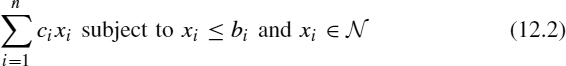
The constrained 2DCSP targets the cutting of a large rectangle S of dimensions L × W in a set of smaller rectangles using orthogonal guillotine cuts: Any cut must run from one side of the rectangle to the other end and be parallel to one of the other two edges. The rectangles produced must belong to one of a given set of rectangle types = {T₁, …, T_n}, where the ith type, T_i, has dimensions l_i × w_i. Associated with each type T_i there is a profit c_i and a demand constraint b_i. The goal is to find a feasible cutting pattern with x_i pieces of type T_i maximizing the total profit:

Wang [24] was the first to make the observation that all guillotine cutting patterns can be obtained by means of horizontal and vertical builds of meta-rectangles. Her idea was exploited by Viswanathan and Bagchi [25] to propose a best-first search A* algorithm (VB). The VB algorithm uses two lists and, at each step, the best build of pieces (or metarectangles) is combined with the best metarectangles already found to produce horizontal and vertical builds. All the approaches to parallelize VB make a special effort to manage the highly irregular computational structure of the algorithm. Attempts to deal with its intrinsically sequential nature inevitably appears either transformed on an excessively fine granularity or any other source of inefficiency [26,27].

The Viswanathan and Bagchi algorithm follows a scheme similar to an A* search, so that implementation with the skeleton is direct. At each moment, the best current build considered must be selected and placed at the left bottom corner of the surface S. Then it must be combined horizontally and vertically with the best builds selected previously (dependent-type branches). That is, the insertion in the open list must be done by order (depending on the value of the estimated total profit). This can be indicated by fixing the option PRIORITY_HIGHER in the features of the open list. The algorithm does dependent branches, so it is necessary to use the best list. The solver finishes the search when the first solution is found. If the upper_bound method has been defined properly, the first solution will be the best solution to the problem. Besides, in this particular case, the skeleton has been tuned to avoid analyzing subproblems similar and worse than others explored previously.

12.5 EXPERIMENTAL RESULTS

For the computational study of the ECC, a set of problem instances with different values of n and M were selected to test the behavior of the solvers provided. For all these instances, the minimum number of errors to correct was set to 1. For the 2DCSP, we have selected some instances from those available in refs. 28 and 29. The experiments were carried out on an Origin 3800 with 160-MIPS R14000 (600-MHz) processors. The compiler used was the MIPSpro v.7.41.

The execution times for the ECC problem obtained with the sequential solver and the one-thread parallel solver are shown in Table 12.1. The comparison of such times reveals the overhead introduced by the shared memory scheme. Due to the problem specification, all nodes generated need to be computed (i.e., the entire search space is explored to ensure achievement of the best solution). So the number of nodes computed for the sequential and parallel executions is always the same. The parallel results obtained with the shared-memory solver are presented in Table 12.2. Parallel times show that some improvements were improved, although the problem behavior does not seem very stable. The total number of nodes computed does not decrease in the parallel executions, so the speedup achieved is obtained by means of the parallel work among threads.

The sequential results obtained for the 2DCSP are presented in Table 12.3. Due to the implementation done, the number of nodes generated is different from the number of nodes computed because the search finishes when the first solution arrives. That leaves nodes in the open list that have been created but will not be explored. Sequential times for the most common test instances in the literature [28] are almost negligible, so some larger instances [29] were selected for the parallel study. Results obtained with the parallel solver are shown in Table 12.4. In the parallel executions, the total number of nodes computed may vary since the search order is altered. When searching in parallel, the global bounds can easily be improved, yielding a decreasing number of nodes computed (e.g., problem instance cat3_2). Although in cases where the bounds are highly accurate, the parallel search may produce some nodes that are not generated in the sequential search (e.g., problem instance cat1_1). In general, the parallel results for the 2DCSP get worse, with more threads participating in the solution. This usually occurs when trying to parallelize fine-grained problems. To provide an idea of the load balancing during the parallel executions, Figure 12.2 is shown. Computation of the nodes is distributed among the master and slave threads. The master leads the exploration order, while the slave threads generate nodes and their corresponding insertions into the local lists. For the ECC problem, the number of nodes computed by each master–slave thread is shown. In this case, all the nodes generated are inserted and computed during the search process. For the 2DCSP, the number of nodes inserted are shown. For this problem, the insertion of a node represents the heavier workload done by each thread (i.e., checking for similarities and duplicated nodes). In general, a fair distribution of nodes is difficult to obtain since it is not only needed to distribute the subproblems fairly to be generated but also those to be inserted. Before doing a certain combination, we are unable to know if it will be valid or not (to be inserted). Anyway, even when a fair balance of the inserted nodes is achieved, it does not mean that the work involved is distributed homogeneously. Due to the internal operation of the parallel solver, it usually ensures a fair distribution of the workload. Although the “number of computed or inserted nodes” is not properly distributed among the threads, the work involved is always balanced. The load balancing is better achieved for fine-grained problems: Every time a thread finishes a node branching, it asks for the next one to be explored.

TABLE 12.1 ECC Sequential Executions

TABLE 12.2 ECC Parallel Executions

TABLE 12.3 2DCSP Sequential Executions

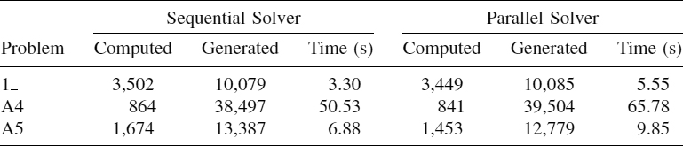
TABLE 12.4 2DCSP Parallel Executions

Figure 12.2 Load balancing: (a) ECC (n = 13, M = 5); (b) 2DCSP (cat3_2).

12.6 CONCLUSIONS

Considering the similarities among many different types of tree searches, an algorithmic skeleton was developed to simplify implementation of these general tree searches. The skeleton provides a sequential and a parallel solver as well as several setup options that make it possible to configure flexible searches. The main contribution is the parallel solver: It was implemented using the shared-memory paradigm. We presented computational results obtained for the implementation of two different complex problems: ECC and 2DCSP.

As we have shown, the synchronization needed to allow the list to reside in shared memory introduces significant overhead to the parallel version. The results seem to be improved when the skeleton executes a search with independent generation of subproblems (i.e., the ECC problem). When it is not necessary to maintain the list ordered and the problem has coarse grain, the threads spend less time looking for work and doing the corresponding synchronization through the list. That makes it possible to obtain lower overhead and better speedup. In such cases, some time improvements are obtained, thanks to the parallel analysis of nodes. The improvements introduced by the parallel solver in the case of the 2DCSP (fine-grained and dependent generation of subproblems) are obtained because the number of nodes generated decreases when more threads collaborate in the problem solution. That is because the update of the best current bound is done simultaneously by all the threads, allowing subproblems to be discarded that in the sequential case have to be inserted and explored.

In any type of tree search, sublinear and superlinear speedups can be obtained since the search exploration order may change in the parallel executions [30–32]. Parallel speedups depend strongly on the particular problem. That is a result of changing the search space exploration order when more than one thread is collaborating in the solution. Anyway, even in cases where the parallel execution generates many more nodes than does sequential execution, the parallel scheme is able to improve sequential times. Synchronization between threads when accessing the global list is a critical point, so the behavior and scalability of the parallel scheme is not completely uniform. As shown, the times (for both problems) in different executions are not very stable. In any case, the parallel results depend strongly on the platform characteristics (compiler, processor structure, exclusive use, etc.).

The main advantage of this tool is that the user can tune all the search parameters to specify many different types of tree searches. In addition, the user gets a sequential and a parallel solver with only simple specification of the problem. Another advantage of the parallel scheme is that the work distribution between the slaves is balanced. The parallel solver works fine for coarse-grained and independent generation-type problems, but for fine-grained problems with dependent generation of subproblems, the synchronization required for sharing the algorithm structures introduces an important overhead to the scheme. For this reason, a more coarse-grained parallelization is being considered to partially avoid such overhead.

Acknowledgments

This work has been supported by the EC (FEDER) and by the Spanish Ministry of Education and Science under the Plan Nacional de I+D+i, contract TIN2005-08818-C04-04. The work of G. Miranda has been developed under grant FPU-AP2004-2290.

REFERENCES

1. A. H. Land and A. G. Doig. An automatic method of solving discrete programming problems. Econometrica, 28(3):497–520, 1960.

2. E. Lawler and D. Wood. Branch-and-bound methods: a survey. Operations Research, 14:699–719, 1966.

3. L. G. Mitten. Branch-and-bound methods: general formulation and properties. Operations Research, 18(1):24–34, 1970.

4. T. Ibaraki. Theoretical comparisons of search strategies in branch-and-bound algorithms. International Journal of Computer and Informatics Sciences, 5(4):315–344, 1976.

5. P. E. Hart, N. J. Nilsson, and B. Raphael. A formal basis for the heuristic determination of minimum cost paths. IEEE Transactions on Systems Science and Cybernetics, SSC-4(2):100–107, 1968.

6. T. Ibaraki. Enumerative approaches to combinatorial optimization (Part I). Annals of Operations Research, 10(1–4):1–342, 1987.

7. D. S. Nau, V. Kumar, and L. Kanal. General branch and bound, and its relation to A* and AO*. Articial Intelligence, 23(1):29–58, 1984.

8. B. Le Cun, C. Roucairol, and TNN Team. BOB: a unified platform for implementing branch-and-bound like algorithms. Technical Report 95/016. Laboratoire PRiSM, Université de Versailles, France, 1995.

9. Y. Shinano, M. Higaki, and R. Hirabayashi. A generalized utility for parallel branch and bound algorithms. In Proceedings of the 7th IEEE Symposium on Parallel and Distributed Processing, 1995, pp. 392–401.

10. S. Tschöke and T. Polzer. Portable parallel branch-and-bound library. PPBB-Lib User Manual, Library Version 2.0. Department of Computer Science, University of Paderborn, Germany, 1996.

11. R. C. Correa and A. Ferreira. Parallel best-first branch-and-bound in discrete optimization: a framework. Solving Combinatorial Optimization Problems in Parallel: Methods and Techniques, vol. 1054 of Lecture Notes in Computer Science, Springer-Verlag, New York, 1996, pp. 171–200.

12. PICO: an object-oriented framework for parallel branch and bound. In Proceedings of the Workshop on Inherently Parallel Algorithms in Optimization and Feasibility and their Applications. Elsevier Scientific, New York, 2000, pp. 219–265.

13. E. Alba et al. MALLBA: A library of skeletons for combinatorial optimization. In Proceedings of Euro-Par, vol. 2400 of Lecture Notes in Computer Science. Springer-Verlag, Berlin, 2002, pp. 927–932.

14. T. K. Ralphs, L. Ladányi, and M. J. Saltzman. A library hierarchy for implementing scalable parallel search algorithms. Journal of Supercomputing, 28(2):215–234, 2004.

15. A. Grama and V. Kumar. State of the art in parallel search techniques for discrete optimization problems. Knowledge and Data Engineering, 11(1):28–35, 1999.

16. V. D. Cung, S. Dowaji, B. Le Cun, T. Mautor, and C. Roucairol. Parallel and distributed branch-and-bound/A* algorithms. Technical Report 94/31. Laboratoire PRiSM, Université de Versailles, France, 1994.

17. V. D. Cung and B. Le Cun. An efficient implementation of parallel A*. In Proceedings of the Canada–France Conference on Parallel and Distributed Computing, 1994, pp. 153–168.

18. G. Miranda and C. León. OpenMP skeletons for tree searches. In Proceedings of the 14th Euromicro Conference on Parallel, Distributed and Network-based Processing. IEEE Computer Society Press, Los Alamitos, CA, 2006, pp. 423–430.

19. J. R. González, C. León, and C. Rodríguez. An asynchronous branch and bound skeleton for heterogeneous clusters. In Proceedings of the 11th European PVM/MPI Users' Group Meeting, vol. 3241 of Lecture Notes in Computer Science. Springer-Verlag, New York, 2004, pp. 191–198.

20. G. Miranda and C. León. An OpenMP skeleton for the A* heuristic search. In Proceedings of High Performance Computing and Communications, vol. 3726 of Lecture Notes in Computer Science. Springer-Verlag, New York, 2005, pp. 717–722.

21. I. Dorta, C. León, and C. Rodríguez. A comparison between MPI and OpenMP branch-and-bound skeletons. In Proceedings of the 8th International Workshop on High Level Parallel Programming Models and Supportive Enviroments. IEEE Computer Society Press, Los Alamitos, CA, 2003, pp. 66–73.

22. R. Hill. A First Course in Coding Theory. Oxford Applied Mathematics and Computing Science Series. Oxford University Press, New York, 1986.

23. C. León, S. Martín, G. Miranda, C. Rodríguez, and J. Rodríguez. Parallelizations of the error correcting code problem. In Proceedings of the 6th International Conference on Large-Scale Scientific Computations, vol. 4818 of Lecture Notes in Computer Science. Springer-Verlag, New York, 2007, pp. 683–690.

24. P. Y. Wang. Two algorithms for constrained two-dimensional cutting stock problems. Operations Research, 31(3):573–586, 1983.

25. K. V. Viswanathan and A. Bagchi. Best-first search methods for constrained two-dimensional cutting stock problems. Operations Research, 41(4):768–776, 1993.

26. G. Miranda and C. León. OpenMP parallelizations of Viswanathan and Bagchi's algorithm for the two-dimensional cutting stock problem. In Parallel Computing 2005, NIC Series, vol. 33, 2005, pp. 285–292.

27. L. García, C. León, G. Miranda, and C. Rodríguez. Two-dimensional cutting stock problem: shared memory parallelizations. In Proceedings of the 5th International Symposium on Parallel Computing in Electrical Engineering. IEEE Computer Society Press, Los Alamitos, CA, 2006, pp. 438–443.

28. M. Hifi. An improvement of Viswanathan and Bagchi's exact algorithm for constrained two-dimensional cutting stock. Computer Operations Research, 24(8):727–736, 1997.

29. DEIS Operations Research Group. Library of instances: two-constraint bin packing problem. http://www.or.deis.unibo.it/research_pages/ORinstances/2CBP.html.

30. B. Mans and C. Roucairol. Performances of parallel branch and bound algorithms with best-first search. Discrete Applied Mathematics and Combinatorial Operations Research and Computer Science, 66(1):57–76, 1996.

31. T. H. Lai and S. Sahni. Anomalies in parallel branch-and-bound algorithms. Communications of the ACM, 27(6):594–602, 1984.

32. A. Bruin, G. A. P. Kindervater, and H. W. J. M. Trienekens. Asynchronous parallel branch and bound and anomalies. In Proceedings of the Workshop on Parallel Algorithms for Irregularly Structured Problem, 1995, pp. 363–377.