 CHAPTER 15
Evolving Rules for Local Time Series Prediction
C. LUQUE, J. M. VALLS, and P. ISASI
Universidad Carlos III de Madrid, Spain
15.1 INTRODUCTION
A time series (TS) is a sequence of values of a variable obtained at successive, in most cases uniformly spaced, intervals of time. The goal is to predict future values of the variable yi using D past values. In other words, the set {y1, …, yD} is used to predict yD + τ, where τ is a nonnegative integer, which receives the name of the prediction horizon. In TS related to real phenomena, a good model needs to detect which elements in the data set can generate knowledge leading to refusing those that are noise. In this work a new model has been developed, based on evolutionary algorithms to search for rules to detect local behavior in a TS. That model allows us to improve the prediction level in these areas.
Previous studies have used linear stochastic models, mainly because they are simple models and their computational burden is low. Autoregressive moving average (ARMA) models using data as to air pressure and water level at Venice have been used to forecast the water level at the Venice lagoon [1]. Following this domain, Zaldívar et al. [2] used a TS analysis based on nonlinear dynamic systems theory, and multilayer neural network models can be found. This strategy is applied to the time sequence of water-level data recorded in the Venice lagoon during the years 1980–1994. Galván et al. [3] used multilayer perceptrons trained using selective learning strategies to predict the Venice lagoon TS. Valls et al. [4] used radial basis neural networks trained with a lazy learning approach applied to the same TS and the well-known Mackey–Glass TS. Following Packard's work to predict dynamic systems [5–7], and using evolutionary algorithms [8–12] to generate prediction rules for a TS, some advanced techniques have been used in this work to obtain better results.
15.2 EVOLUTIONARY ALGORITHMS FOR GENERATING PREDICTION RULES
In some domains, especially in the case of natural phenomena, the use of machine learning techniques is faced with certain problems. Usually, machine learning techniques, especially evolutionary algorithms, base their learning process on a set of examples. If these examples are distributed fundamentally throughout certain values, the learning process will focus on this range, considering the remaining values as noise. This fact is positive for some domains, but it becomes a disadvantage in others. For example, in the case of stock market or tide prediction, to mention two very different domains, most existing measures are over average values. On a few occasions, great increases or decreases take place. Nevertheless, those situations are indeed the situations that have more importance from the point of view of the prediction task. Our approach is based on finding rules that represent both the usual and atypical behaviors of the TS, to enable us to predict future values of the series. These rules will be obtained using an evolutionary algorithm.
To avoid the generalization problem, a Michigan approach has been implemented [13] in the evolutionary algorithm, using a steady-state strategy. In the Michigan approach, the solution to the problem is the total population instead of the individual that best fits. This allows us to evolve rules for common behaviors of the problem but also allows atypical behaviors. Doing that, we pay attention to those unusual behaviors which in other cases would be considered as noise.
Due to the fact that each rule is evaluated using only examples associated with it, it is only locally or partially applicable. This local characteristic allows the system to use specific rules for particular situations. On the other hand, this method does not assure that the system will make a prediction for all the TS. A balance must be found between system performance and the percentage of prediction.
15.3 EXPERIMENTAL METHODOLOGY
The approach suggested in this chapter is based on the generation of rules for making predictions. The steps, divided into encoding, initialization, evolution, and prediction, are explained in detail in this section.
15.3.1 Encoding
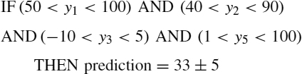
The first step consists of fixing a value for the constant D that represents the number of consecutive time instants used to make the prediction. For example, if D = 5, a rule could be a condition such as “if the value of the variable at time unit 1 is smaller than 100 and bigger than 50, at time unit 2 is smaller than 90 and bigger than 40, at time unit 3 is smaller than 5 and bigger than −10, at time unit 5 is smaller than 100 and bigger than 1, the measure at time unit 5 + τ will be 33 with an expected error of 5.” This rule could be expressed as
In Figure 15.1 a graphical representation of a rule is shown. For a rule (R), a conditional part (CR) and a predicting part (PR) are defined. The conditional part consists of a set of pairs of intervals ![]() , where each
, where each ![]() is an interval
is an interval ![]() ,
, ![]() being the lower limit and
being the lower limit and ![]() the upper limit for the ith input data. The predicting part is composed of two values: the prediction value and the expected error, PR = {pR, eR}. The conditional part could include void values (∗), which means that the value for this interval is irrelevant; that is, we don't care which value it has. The previous rule is encoded as (50, 100, 40, 90, − 10, 5, ∗, ∗, 1, 100, 33, 5).
the upper limit for the ith input data. The predicting part is composed of two values: the prediction value and the expected error, PR = {pR, eR}. The conditional part could include void values (∗), which means that the value for this interval is irrelevant; that is, we don't care which value it has. The previous rule is encoded as (50, 100, 40, 90, − 10, 5, ∗, ∗, 1, 100, 33, 5).
In this way, all the individuals in our evolutionary strategy can be encoded as vectors of real numbers of size 2 × D + 2, D being the number of time units used for prediction. Genetic operators can be used to generate new rules from an initial population. To do that we need to define a crossover process. We select two rules in the population, and they produce a new offspring rule. This offspring will inherit his genes from his parents, each gene being an interval Ij. For each i < D the offspring can inherit two genes (one from each parent) with the same probability. This type of crossover is known as uniform crossover. This offspring will not inherit the values for “prediction” and “error,” as we can see in the following example:

Figure 15.1 Graphical representation of a rule.

An example of this process is shown graphically in Figure 15.2. Once generated, an offspring may suffer an interval mutation. This event takes place with a 10% probability for each new individual. Should the individual be selected, one of its intervals will be altered.
Mutations over the interval (LL, UL) are shown in Table 15.1. All these mutations have the same probability of being selected. R(x, y) means a random value between x and y with x < y, and W means the 10% of the width of the interval defined by (LL, UL). In other words, W = 0.1(UL − LL). Obviously, the transformation of (LL,UL) into (LL′,UL′) must fit the condition LL′ < UL′. Figure 15.3 summarizes these alternatives.
For each rule, several values are needed for the prediction made for that rule, and its expected accuracy or precision. As already mentioned, these values are not inherited from parents but must also be computed. With R representing an individual, the process to obtain the prediction and error values for R is the following:

Figure 15.2 Crossover.
| Name | Transformation |
| New random value | (LL, UL) → (R(0, 1), R(0, 1)) |
| Null condition | (LL, UL) → (∗, ∗) |
| Enlarge | (LL, UL) → (LL−R(0, 1)W, UL + R(0, 1)W) |
| Shrink | (LL, UL) → (LL + R(0, 1)W, UL − R(0, 1)W) |
| Move up | (LL, UL) → (LL + cW, UL + cW) c = R(0, 1) |
| Move down | (LL, UL) → (LL − cW, UL − cW) c = R(0, 1) |

Figure 15.3 Mutation.
- We must calculate the set of points of the TS S = {x1, x2, …, xk, …, xm} such that it fits the conditional part of the rule R. This subset will be called CR(S) and is defined as
where
 and the vector
  fits CR if all its values fall inside the intervals of the rule:
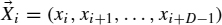
 - Once CR(S) is calculated, the next step consists of determining the output for the prediction horizon τ for each point. This value is vi = xi + D − 1 + τ.
- This new value is added to the vector as a new component, so we have
 , where
  is defined as
- The prediction pR for the rule R is calculated by means of a linear regression with all the vectors in the set
 . To do that it is necessary to calculate the coefficients of the regression
  , which define the hyperplane that better approximates the set of points . Let
  be the estimated value obtained by regression at the point , which follows
- Thus, the estimated error value for the rule, eR, is defined as

Therefore, each individual represents a rule able to predict the series partially. The set of all individuals (all the rules) defines the prediction system. Nevertheless, zones of the series that do not have any associated rule could be found. In this case the system cannot make a decision in this region. It is desirable, and it is an objective of this work, to make the unpredicted zone as small as possible, always being careful not to decrease the predictive ability of the system for other regions. For this objective, the work tries to find automatically, at the same time that the rules are discovered, how to divide the problem space into independent regions, where different and ad hoc sets of rules could be applied without being affected by distortions that general rules have in some specific zones of the problem space.
This could be summarized in searching sets of rules that allow equilibrium between generalization and accuracy: rules that could achieve the best predictive ability in as many regions as possible but being as general as possible at the same time. Our system must therefore look for individuals that on the training set predict the maximum number of points with the minimum error. Following this idea, the fitness function for an individual R is defined in this way:
IF ((NR>1) AND (eR<EMAX)) THEN
      fitness = (NR*EMAX) - eR
ELSE
   fitness = f_min
where NR is the number of points of the training set that fit the condition CR [i.e., NR = cardinal(CR(S))]. EMAX is a parameter of the algorithm that punishes those with a maximum absolute error greater than EMAX. fmin is a minimum value assigned to those whose rule is not fitted at any point in the training set. This means that if the number of examples accomplished by a rule is low, or the error in that set is big, the fitness will be the worst value, being the relative error as fitness otherwise.
The goal of this fitness function is to establish a balance between individuals whose prediction error is the lowest possible, and at the same time, the number of points of the series in which it makes a prediction [the number of points of CR(S)] is the highest possible, that is, to reach the maximum possible generalization level for each rule.
15.3.2 Initialization
The method designed tends to maintain the diversity of the individuals in the population as well as its capacity to predict different zones of the problem space. But the diversity must exist previously. To do that, a specific procedure of population initialization has been devised. The main idea of this procedure is to make a uniform distribution throughout the range of possible output data. For example, in the case of Venice lagoon tide prediction, the output ranges from −50 to 150 cm. If the population has 100 individuals, the algorithm will create 100 intervals of 2 cm width, and in this way all the possible values of the output are included. The initialization procedure includes a rule for each interval mentioned previously, so intervals will have a default rule at the beginning of the process. The initialization procedure for an interval I has the following steps:
- Select all the training patterns whose output belongs to I.
- Determine a maximum and a minimum value for each input variable of all the pattern selected in step 1. For example, if the patterns selected are (1,2,3), (2,2,2), (5,1,5), and (4,5,6), the maximum values should be 5, 5, and 6 for the first, second, and third input variables. So the minimum values should be 1, 1, and 2.
- Those maximum and minimum values define the values assigned to the rule for each input variable. This rule's prediction is set as the mean of the output value of the patterns selected in step 1.
This procedure will produce very general rules, so they will cover all the prediction space. From this set of rules, the evolutionary algorithm will evolve new, more specific rules, improving both the general predictive ability of the entire system and the prediction level in each specific zone of the space defined by each rule.
15.3.3 Evolution of Rules
Basically, the method described in this chapter uses a Michigan approach [6] with a steady state strategy. That means that at each generation two individuals are selected proportionally to the fitness function. We choose a tournament selection of size 3 as the selection operator. Those parents produce only one offspring by crossover. Then the algorithm replaces the individual nearest the offspring in phenotypic distance (i.e. it looks for the individual in the population that make predictions on similar zones in the prediction space). The offspring replaces the individual selected if and only if its fitness is higher; else the population does not change. This replacement method is used primarily in crowding methods [14]. Those methods try to maintain a diverse population to find several solutions to the problem. In the case of study in this chapter, this approach is justified by the fact that we are looking for several solutions to cover the space of prediction as widely as possible so that rules generated could predict the highest number of situations. Moreover, the diversity of the solutions allows the generation of rules for specific highly special situations. The pseudocode of the entire system is shown in Algorithm 15.1.
15.3.4 Prediction
The stochastic method defined previously obtains different solutions in different executions. After each execution the solutions obtained at the end of the process are added to those obtained in previous executions. The number of executions is determined by the percentage of the search space covered by the rules. The set of all the rules obtained in the various executions is the final solution of the system. Once the solution is obtained, it is used to produce outputs to unknown input patterns. This is done following the next steps:
- For each input pattern, we look for the rules that this pattern fits.
- Each rule produces an output for this pattern.
- The final system output (i.e., the prediction of the system) is the mean of the outputs for each pattern.
Those steps are summarized in Figure 15.4. In this case, when an unknown pattern is received, it may fit some of the rules in the system. In the example, rules 1, 2, 3, 5, 6, 8, 9, and 10 are fitted. Each fitted rule makes a prediction, so we have eight different predictions. To obtain the final prediction of the system for that pattern, the mean of all predictions is chosen as the definitive prediction for that pattern. If the pattern doesn't fit any rule, the system produces no prediction.
15.4 EXPERIMENTS
The method has been applied to three different domains: an artificial domain widely used in the bibliography (Mackey–Glass series) and two TSs corresponding to natural phenomena: the water level in Venice lagoon and the sunspot TS.
15.4.1 Venice Lagoon TS
One real-world TS represents the behavior of the water level at the Venice lagoon. Unusual high tides result from a combination of chaotic climatic elements with the more normal, periodic tidal systems associated with a particular area. The prediction of high tides has always been a subject of intense interest, not only from a human point of view but also from an economic one, and the water level of the Venice lagoon is a clear example of these events [1,15]. The most famous example of flooding in the Venice lagoon occurred in November 1966, when the water rose nearly 2 meters above the normal level. This phenomenon, known as high water, has spurred many efforts to develop systems to predict the sea level in Venice, mainly for the prediction of the high-water phenomenon [16]. Different approaches have been developed for the purpose of predicting the behavior of sea level at the lagoon [16,17]. Multilayer feedforward neural networks used to predict the water level [2] have demonstrated some advantages over linear and traditional models. Standard methods produce very good mean predictions, but they are not as successful for those unusual values. For the experiments explained above, the following values for the variables τ and D have been used: D = 24 and τ = 1, 4, 12, 24, 28, 48, 72, 96. That means that the measures of the 24 consecutive hours of the water level have been used to predict the water level, measured in centimeters: 1, 4, 12, … hours later.
Algorithm 15.1 Algorithm of Local Rules

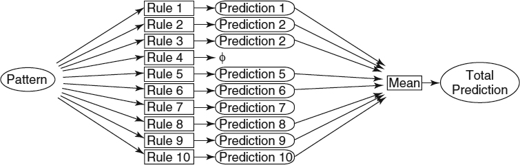
Figure 15.4 Schema of the prediction.
The results from the experiments using the rule system (RS) are shown in Table 15.2, and the results obtained by other well-known machine learning algorithms (MLAs), in Table 15.3. The WEKA tool was used to perform a comparison with the MLA. Those experiments use a training set of patterns created by the first 5000 measures and a validation set of 2000 patterns. The populations of 100 persons evolved within 75,000 generations. The rules used as input 24 consecutive hours of the water level. The value “percentage of prediction” is the percentage of points in the validation set such that there is a prediction for it by at least one rule. No rule made a prediction for the remainder of the validation set. Columns SMO-Reg, IBK, LWL, Kstar, M5Rules, M5p, RBNN (radial basis neural networks), Perceptron NN, and Conjunctive Rules show the error obtained by those MLAs. The error measure used in those experiments is the root-mean-squared error (RMSE), normalized by the root of the variance of the output (NRMSE). Those error measures are defined as
TABLE 15.2 NRMSE and Percentage of Prediction Obtained by the RS for the Venice Lagoon TS
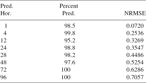
TABLE 15.3 NRMSE Obtained by Other MLAs for the Venice Lagoon TS

For those experiments, the objective was to maximize the percentage of validation set data predicted, avoiding a high mean error. It is interesting to observe that when the prediction horizon increases, the percentage of prediction does not diminish proportionally. Thus, the system seems to be stable to variations in the prediction horizon. This property seems very interesting, because it shows that the rules are adapted to the special and local characteristics of the series.
Studying Tables 15.2 and 15.3, it is important to remark that the prediction accuracy of the rule system outperforms most of the algorithms, being the percentage of prediction data very close to 100%. The SMO-Reg algorithm is the only one that improves most of the rule system results in most of the horizons for that problem. M5Rules and M5P algorithms' results are pretty close and slightly worse than the RS results. Real tide values and the prediction obtained by the RS with horizon 1 for a case of unusual high tide are compared in Figure 15.5. It can be seen how good the predicted value is, even for unusual behaviors.
15.4.2 Mackey–Glass TS
The Mackey–Glass TS is an artificial series widely used in the domain of TS forecasting [18–20] because it has specially interesting characteristics. It is a chaotic series that needs to be defined in great detail. It is defined by the differential equation

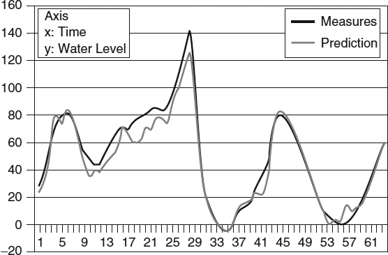
Figure 15.5 Prediction for an unusual tide with horizon 1.
As in refs. 18–20, the values a = 0.2, b = 0.1, and λ = 17 were used to generate the TS. Using Equation 15.8, 30,000 values of the TS are generated for each horizon. The initial 4000 samples are discarded to avoid the initialization transients. With the remaining samples, the training set used was composed of the points corresponding to the time interval [5000, 25,000]. The test set was composed of the samples [4000, 5000]. All data points are normalized in the interval [0, 1].
The results for the rule system algorithm are given in Table 15.4. For the same prediction horizon, the results of the algorithms IBK, LWL, KStar, M5Rules, M5p, Perceptron Neural Networks, Radial Basis Neural Networks, and Conjunctive Rule implemented in WEKA can be seen in Table 15.5. The error used for comparison is NRMSE (normalized root-mean-squared error). In both cases, the rule system improves over the result of most of the other algorithms (except IBK and KStar). This suggests that we have a better level of prediction for the difficult regions of the TS. The percentage of prediction for the test set (more than 75%) induces us to think that the discarded elements were certainly inductive of a high level of errors, since their discard allows better results than those obtained in the literature.
TABLE 15.4 NRMSE and Percentage of Prediction Obtained by the RS for the Mackey–Glass TS

TABLE 15.5 NRMSE Obtained by Other MLA for the Mackey–Glass TS

15.4.3 Sunspot TS
This TS contains the average number of sunspots per month measured from January 1749 to March 1977. These data are available at http://sidc.oma.be (“RWC Belgium World Data Center for the Sunspot”). That chaotic TS has local behaviors, noise, and even unpredictable zones using the archived knowledge. In Table 15.6 we can see the error and percentage of prediction obtained by the RS for different prediction horizons. Table 15.7 shows the results obtained for the same horizons by other well-known MLAs: SMO-Reg, IBK, LWL, KStar, M5Rules, M5p, and Conjunctive Rules are implemented WEKA. The results for Multilayer Feedforward NN and Recurrent NN have been obtained from Galván and Isasi [21]. The error measure used in both tables is defined as

In all cases the experiments were done using the same data set: from January 1749 to December 1919 for training, and from January 1929 to March 1977 for validation, standardized in the [0, 1] interval; in all cases, 24 inputs were used. In all cases the algorithm explained in this chapter (RS) improves over the results obtained by the other MLA, with a percentage of prediction very close to 100%. That fact suggests that we may obtain an even lower error if we prefer to sacrifice this high percentage of prediction. A deeper study of the results confirms the ability of this system to recognize, in a local way, the peculiarities of the series, as in the previous domains.
TABLE 15.6 NRMSE and Percentage of Prediction Obtained by the RS for the Sunspot TS

TABLE 15.7 NRMSE Obtained by Other MLA for the Sunspot TS

15.5 CONCLUSIONS
In this chapter we present a new method based on prediction rules for TS forecasting, although it can be generalized for any problem that requires a learning process based on examples. One of the problems in the TS field is the generalization ability of artificial intelligence learning systems. On the one hand, general systems produce very good predictions over all the standard behaviors of the TS, but those predictions usually fail over extreme behaviors. For some domains this fact is critical, because those extreme behaviors are the most interesting.
To solve this problem, a rule-based system has been designed using a Michigan approach, tournament selections, and replacing new individuals by a steady-state strategy. This method includes a specific initialization procedure (Section 15.3.2) and a process designed to maintain the diversity of the solutions. This method presents the characteristic of not being able to predict the entire TS, but on the other hand, it has better accuracy, primarily for unusual behavior. The algorithm can also be tuned to attain a higher prediction percentage at the cost of worse prediction results.
Results show that for special situations, primarily for unusual behaviors (high tides, function peaks, etc.), the system is able to obtain better results than do the previous works, although the mean quality of the predictions over the entire series is not significantly better. Therefore, if it is possible, the system can find good rules for unusual situations, but it cannot find better rules for standard behaviors of the TS than can the previous works, where standard behaviors indicates behaviors that are repeated more often along the TS.
Another interesting characteristic of the system is its ability to find regions in the series whose behavior cannot be generalized. When the series contains regions with special particularities, the system cannot only localize them but can build rules for a best prediction of them. The method proposed has been devised to solve the TS problem, but it can also be applied to other machine learning domains.
Acknowledgments
This work has been financed by the Spanish-funded research MCyT project TRACER (TIC2002-04498-C05-04M) and by the Ministry of Science and Technology and FEDER contract TIN2005-08818-C04-01 (the OPLINK project).
REFERENCES
1. E. Moretti and A. Tomasin. Un contributo matematico all'elaborazione previsionale dei dati di marea a Venecia. Boll. Ocean. Teor. Appl. 2:45–61, 1984.
2. J. M. Zaldívar, E. Gutiérrez, I. M. Galván, and F. Strozzi. Forecasting high waters at Venice lagoon using chaotic time series analysis and nonlinear neural networks. Journal of Hydroinformatics, 2:61–84, 2000.
3. I. M. Galván, P. Isasi, R. Aler, and J. M. Valls. A selective learning method to improve the generalization of multilayer feedforward neural networks. International Journal of Neural Systems, 11:167–157, 2001.
4. J. M. Valls, I. M. Galván, and P. Isasi. Lazy learning in radial basis neural networks: a way of achieving more accurate models. Neural Processing Letters, 20:105–124, 2004.
5. T. P. Meyer and N. H. Packard. Local forecasting of high-dimensional chaotic dynamics. In M. Casdagli and S. Eubank, eds., Nonlinear Modeling and Forecasting. Addison-Wesley, Reading, MA, 1990, pp. 249–263.
6. M. Mitchell. An Introduction to Genetic Algorithms. MIT Press, Cambridge, MA, 1996, pp. 55–65.
7. N. H. Packard. A genetic learning algorithm for the analysis of complex data. Complex Systems, 4:543–572, 1990.
8. D. B. Fogel. An introduction to simulated evolutionary optimization. IEEE Transactions on Neural Networks, 5(1):3–14, 1994.
9. T. Bäck and H. P. Schwefel. Evolutionary algorithms: some very old strategies for optimization and adaptation. In Proceedings of the 2nd International Workshop Software Engineering, Artificial Intelligence, and Expert Systems for High Energy and Nuclear Physics, 1992, pp. 247–254.
10. J. H. Holland. Adaptation in Natural and Artificial Systems. University of Michigan Press, Ann Arbor, MI, 1975.
11. K. A. De Jong, W. M. Spears, and F. D. Gordon. Using genetic algorithms for concept learning. Machine Learning, 13:198–228, 1993.
12. C. Z Janikow. A knowledge intensive genetic algorithm for supervised learning. Machine Learning, 13:189–228, 1993.
13. L. B. Booker, D. E. Goldberg, and J. H. Holland. Classifier systems and genetic algorithms. Artificial Intelligence, 40:235–282, 1989.
14. K. A. De Jong. Analysis of the behavior of a class of genetic adaptive systems. Ph.D. thesis, University of Michigan, 1975.
15. A. Michelato, R. Mosetti, and D. Viezzoli. Statistical forecasting of strong surges and application to the lagoon of Venice. Boll. Ocean. Teor. Appl., 1:67–76, 1983.
16. A. Tomasin. A computer simulation of the Adriatic Sea for the study of its dynamics and for the forecasting of floods in the town of Venice. Computer Physics Communications, 5–51, 1973.
17. G. Vittori. On the chaotic features of tide elevation in the lagoon Venice. In Proceedings of the 23rd International Conference on Coastal Engineering (ICCE'92), 1992, pp. 4–9.
18. M. C. Mackey and L. Glass. Oscillation and chaos in physiological control systems. Science, 197:287–289, 1997.
19. J. Platt. A resource-allocating network for function interpolation. Neural Computation, 3:213–225, 1991.
20. L. Yingwei, N. Sundararajan, and P. Saratchandran. A sequential learning scheme for function approximation using minimal radial basis function neural networks. Neural Computation, 9:461–478, 1997.
21. I. M. Galván and P. Isasi. Multi-step learning rule for recurrent neural models: an application to time series forecasting. Neural Processing Letters, 13:115–133, 2001.
Optimization Techniques for Solving Complex Problems, Edited by Enrique Alba, Christian Blum, Pedro Isasi, Coromoto León, and Juan Antonio Gómez
Copyright © 2009 John Wiley & Sons, Inc.