 CHAPTER 13
Tools for Tree Searches: Dynamic Programming
C. LEÓN, G. MIRANDA, and C. RODRÍGUEZ
Universidad de La Laguna, Spain
13.1 INTRODUCTION
The technique known as dynamic programming (DP) is analogous to divide and conquer. In fact, it can be seen as a reformulation of the divide-and-conquer (DnC) technique. Consequently, it aims at the same class of problems. Dynamic programming usually takes one of two approaches:
1. Top-down approach. The problem is broken into subproblems, and these subproblems are solved, but (and this is how it differs from divide and conquer) a memory cache (usually, a multidimensional data structure) is used to remember the mapping between subproblems and solutions. Before expanding any subproblem, the algorithm checks to see if the subproblem is in such a cache. Instead of repeating the exploration of the subtree, the algorithm returns the stored solution if the problem has appeared in the past.
2. Bottom-up approach. Subproblems are solved in order of complexity. The solutions are stored (in a multidimensional data structure which is the equivalent of the one used in the top-down approach). The solutions of the simpler problems are used to build the solution of the more complex problems.
From this description follows the main advantages and disadvantages of dynamic programming: There is an obvious gain when the divide-and-conquer search tree is exponential, and subproblems with the same characterization appear again and again. DP fails when there are no repetitions or even though there are, the range of subproblems is too large to fit in computer memory. In such cases the memory cache multidimensional data structure grows beyond the limits of the largest supercomputers.
13.2 TOP-DOWN APPROACH
Dynamic programming is strongly related to a general-purpose technique used to optimize execution time, known as memoization. When a memoized function with a specific set of arguments is called for the first time, it stores the result in a lookup table. From that moment on, the result remembered will be returned rather than recalculated. Only pure functions can be memoized. A function is pure if it is referentially transparent: The function always evaluates the same result value given the same arguments. The result cannot depend on any global or external information, nor can it depend on any external input from I/O devices.
The term memoization derives from the Latin word memorandum (to be remembered) and carries the meaning of turning a function f : X1 × X2 → Y into something to be remembered. At the limit, and although it can be an unreachable goal, memoization is the progressive substitution of f by an associative representation of the multidimensional table:
{(x1, x2, y) ∈ X1 × X2 × Y such that y = f (x1, x2)}
So instead of computing f (x1, x2), which will usually take time, we will simply access the associated table entry f[x1][x2]. Memoization trades execution time in exchange for memory cost; memoized functions become optimized for speed in exchange for a higher use of computer memory space.
Some programming languages (e.g., Scheme, Common Lisp, or Perl) can automatically memoize the result of a function call with a particular set of arguments. This mechanism is sometimes referred to as call by need. Maple has automatic memoization built in.
The following Perl code snippet (to learn more about Perl and memoization in Perl see refs. 1 and 2), which implements a general-purpose memoizer, illustrates the technique (you can find the code examples in ref. 3):
 1 sub memoize {
 2   my $func = shift;
 3
 4   my %cache;
 5   my $stub = sub {
 6      my $key = join ’,’, @_;
 7      $cache{$key} = $func->(@_) unless exists $cache{$key};
 8      return $cache{$key};
 9   };
10   return $stub;
11 }
The code receives in $func the only argument that is a reference to a function (line 2). The call to the shift operator returns the first item in the list of arguments (denoted by @_). A reference to a memoized version of the function is created in $stub (lines 5 to 9). The new function uses a hash %cache to store the pairs evaluated. The unique key for each combination of arguments is computed at line 6. The function arguments in @_ are coerced to strings and concatenated with commas via the join operator in such a way that different combinations of arguments will be mapped onto different strings. The original function is called only if it is the first time for such a combination. In such a case, the result of the call $func-> (@_) is stored in the cache (line 7). The entry will then be used by subsequent calls. Finally, memoize returns the reference to the memoized version of $func (line 10).
To see memoize working, let us apply it to a 0–1 knapsack problem with capacity C and N objects. The weights will be denoted wk and the profits pk. If we denote by fk, c the optimal value for the subproblem considering objects {0, …, k} and capacity c, the following recursive equation holds:
The following Perl subroutine uses Equation 13.1 to solve the problem:
sub knap {
  my ($k, $c) = @_;
  my @s;

  return 0 if $k < 0;
  $s[0] = knap($k-1, $c);
  if ($w[$k] < = $c) {
    $s[1] = knap($k-1, $c-$w[$k])+$p[$k];
  }
  return max(@s);
 }
The following program benchmarks 1000 executions of the divide-and-conquer version versus the top-down memoized dynamic programming version (the function referenced by $mknap, line 7):
$ cat -n memoizeknap.pl
 1  #!/usr/bin/perl -I../lib -w
 2  use strict;
 3  use Benchmark;
 4  use Algorithm::MemoizeKnap;
 5  use List::Util qw(max sum);
 6
 7  my $mknap = memoize(&knap);
 8
 9  my $N = shift || 12;
10  my $w = [ map { 3 + int(rand($N-3)) } 1..$N ];
11  my $p = [ map { $_ } @$w ];
12  my $C = int(sum(@$w)/3);
13
14  set($N, $C, $w, $p);
15
16  my ($r, $m);
17  timethese(1000, {
18    recursive => sub { $r = knap($N-1, $C) },
19    memoized  => sub { $m = $mknap->($N-1, $C) },
20    }
21  );
22
23  print “recursive = $r, memoized = $m
”;
The results are overwhelming: The CPU time for the DP version is negligible while the divide-and-conquer approach takes almost 4 seconds:
$ ./memoizeknap.pl
Benchmark: timing 1000 iterations of memoized, recursive…
  memoized:  0 wallclock secs (0.00 usr + 0.00 sys = 0.00 CPU)
 recursive: 4 wallclock secs (3.75 usr + 0.00 sys = 3.75 CPU)
recursive = 23, memoized = 23
The reason for such success is this: While the divide-and-conquer approach explores a search tree with a potential number of 2N nodes, the memoized (dynamic programming) version never explores more than N × C nodes. Since ![]() , it follows that the same attribute values, ($k, $c), appear again and again during exploration of the nodes of the DnC search tree.
, it follows that the same attribute values, ($k, $c), appear again and again during exploration of the nodes of the DnC search tree.
The contents of this section can be summarized in an equation and a statement:
- Top-down dynamic programming = divide and conquer + memoization
- Apply dynamic programming when the attributes of the nodes in the divide-and-conquer search tree have a limited variation range, which is much smaller than the size of the search tree. Such size variation must fit into the computer memory.
13.3 BOTTOM-UP APPROACH
The bottom-up approach reproduces a traversing of the divide-and-conquer search tree from the leaves to the root. Subproblems are sorted by complexity in such a way that when a subproblem is processed, all the subproblems from which it depends have already being solved. The solutions of such subproblems are then combined to find the solution of the current subproblem. The new solution is stored in the dynamic programming table to be used later during resolution of the subproblems that depend on the current subproblem. Each subproblem is considered only once. A bottom-up DP algorithm is determined by these methods:
- init_table: initializes the DP table with the values for nondependant states.
- next: an iterator. Traverses the directed acyclic graph of the states (also called iteration space) in an order that is compatible with the dependence graph (i.e., a topological sort). Expressed in divide-and-conquer terms: The children are visited before their father.
- combine: equivalent of the homonymus divide-and-conquer method. Therefore, it returns the solution for the current state/subproblem in terms of its children.
- table(problem, sol): updates the entry of the dynamic programming table for subproblem problem with the solution specified in sol.
The following Perl code (see ref. 3) shows a generic bottom-up dynamic programming solver (method run):
sub run {
  my $dp = shift;

  $dp->init_table;
  while (my $s = $dp->next) {
    $dp->table($s, $dp->combine($s));
  }
 }
The following code solves the 0–1 knapsack problem by instantiating all the attributes enumerated in the former list. The combine method simply mimics the dynamic programming equation:
fk,c = max{fk−1,c, fk−1,c−wk + pk if c > wk}
sub combine {
 my $dp = shift;
 my $state = shift;

  return max($dp->children($state));
}
The auxiliar method children returns the children of the current state:
sub children {
  my $dp = shift;
  my ($k, $c) = @{shift()};

  my $wk = $dp->{w}[$k];
  my $pk = $dp->{p}[$k];
  my @s;
  $s[0] = $dp->table([$k-1, $c]);
  $s[1] = $pk+$dp->table([$k-1, $c-$wk]) if $c >= $wk;

  return @s;
 }
The method init_table populates the first row corresponding to the optimal values f0, c, = p0 if c > w0 and 0 otherwise:
sub init_table {
  my $dp = shift;
  my @table;

  my $C = $dp->{C};
  my $w0 = $dp->{w}[0];
  my $p0 = $dp->{p}[0];
  for(my $c = 0; $c <= $C; $c++) {
    $table[0][$c] = ($w0 <= $c)? $p0 : 0;
  }
  $dp->{table} = @table;
 }
The iterator next traverses the iteration space in an order that is compatible with the set of dependencies: index [$k, $c] must precede indices [$k+1,$c] and [$k+1, $c+$w[$k]]:
{
 my ($k, $c) = (1, 0);

 sub next {
   my $dp = shift;

   my ($C, $N) = ($dp->{C}, $dp->{N});

   return [$k, $c++] if $c <= $C;
   $k++;
   return [$k, $c = 0] if ($k < $N);
   return undef;
 }
}
Once the DP bottom-up algorithm has computed the dynamic table, the method solution traverses the table backward to rebuild the solution:
subsolution {
  my $dp = shift;

  my @sol;

  my ($C, $N) = ($dp->{C}, $dp->{N});
  my $optimal = $dp->table([$N-1, $C]);

  # Compute solution backward
  for(my $k = $N-1, my $c = $C; $k >= 0; $k--) {
    my @s = $dp->children([$k, $c]);
    if (max(@s) == $s[0]) {
      $sol[$k] = 0;
    }
    else {
      $sol[$k] = 1;
      $c -= $dp->{w}[$k];
    }
  }
  $dp->{optimal} = $optimal;
  $dp->{solution} = @sol;  # reference to @sol
  return ($optimal, @sol)
 }
13.4 AUTOMATA THEORY AND DYNAMIC PROGRAMMING
In DP terminology the divide-and-conquer subproblems become states. We liberally mix both terms in this chapter. A bit more formally, we establish in the set of nodes of the divide-and-conquer search tree the equivalence relation which says that two nodes are equivalent if they share the same attributes1:
The dynamic programming states are actually the equivalence classes resulting from this equivalence relation. That is, states are the attributes stored in the nodes. As emphasized in the Section 13.3, the most relevant difference between DP and DnC is that nodes with the same attributes are considered only once. A consequence of establishing this equivalence between nodes is that the search space is no longer a tree but a directed acyclic graph (Figure 13.1).

Figure 13.1 Divide-and-conquer nodes with the same attribute are merged: (a) the search tree becomes a DAG (labels inside the nodes stand for attributes); (b) in bottom-up DP the traversing is reversed.
The shape of the DAG in Figure 13.1 suggests a finite automaton. Edges correspond to transitions. An initial state q0 can be added that represents the absence of decisions. In many cases the problem to solve using DP is an optimization problem.2
in which the set of constraints S is modeled as a language; that is, S ⊂ Σ*, where Σ is a finite alphabet of symbols called decisions. The elements of Σ* are called policies. A policy x ∈ Σ* is said to be feasible if x ∈ S.
A large subset of the set of dynamic programming algorithms for optimization problems can be modeled by superimposing a cost structure to a deterministic finite automaton (DFA).
Definition 13.1 An automaton with costs is a triple Π = (M, μ, ξ0) where:
- M = (Q, Σ, q0, δ, F) is a finite automaton. Q denotes the finite set of states, Σ is the finite set of decisions, δ: Q × Σ → Q is the transition function, q0 ∈ Q is the initial state, and F ⊂ Q is the set of final states.
- μ: R × Q × Σ → R is the cost function, where R denotes the set of real numbers. The function μ is nondecreasing in its first argument:

- ξ0 ∈ R is the setup cost of the initial state q0.
The transition function δ: Q × Σ → Q can be extended to the set of policies δ: Q × Σ* → Q following these two formulas:
- δ(q,
 ) = q for all q.
 - δ(q, xa) = δ(δ(q, x), a) for all q and for all a.
The notation δ(x) = δ(q0, x) is also common. Observe that with this formulation, the children of a given node q in the DnC search tree are δ−1(q) = {q′ ∈ Q/δ(q′, a) = q, ∃a ∈ Σ}.
The cost function μ can also be extended to policies using these two inductive equations:
 for ξ ∈ R and q ∈ Q.
- μ(ξ, q,xa) = μ(μ(ξ, q, x), δ(q, x), a) for ξ ∈ R, q ∈ Q, x ∈ Σ* and a ∈ Σ.
The notation μ(x) = μ(ξ0, q0, x) is also used.
Definition 13.2 A finite automaton with costs Π = (M, μ, ξ0) represents the optimization problem
min f (x) subject to x ∈ S
if and only if it satisfies:
- The language accepted by the automaton M is the set of feasible solutions S, that is,
L(M) = {x ∈ Σ*/δ(x) ∈ F} = S
- For any feasible policy x ∈ S, f (x) = μ(x) holds.
Definition 13.3 For any state q we define G(q) as the optimal value of any policy leading from the start state q0 to q [i.e., G(q) = min{μ(x)/x ∈ Σ* and δ(x) = q} assuming that q is reachable; otherwise, G(q) = ∞].
With these definitions it is now possible to establish the dynamic programming equations:

Bellman's Optimality Principle The principle of optimality introduced by R. Bellman can now be summarized by saying that if x ∈ S is an optimal policy between states q1 and q2,
δ(q1, x) = q2 and μ(q1, x) ≤ μ(q1, u) ∀u ∈ Σ*/δ(q1, u) = q2
then any substring/subpolicy y of x = zyw is also optimal between states q3 = δ(q1, z) and q4 = δ(q1, zy).
μ(q3, y) ≤ μ(q3, u) ∀u ∈ Σ*/δ(q3, u) = q4
Not any DP optimization algorithm can be modeled through a finite automaton with costs. An example is the multiplication parenthesization problem (MPP):
Definition 13.4 In the MPP we have n matrices Mi, i = 1, …, n. Matrix Mi has dimensions ci−1 × ci. The number of operations when doing the product of the n matrices,
P = M1 × M2 × ··· × Mn
depends on the way they are associated. For example, let c0 = 10, c1 = 20, c2 = 50, c3 = 1, and c4 = 100. Then evaluation of P = M1 × (M2 × (M3 × M4)) requires the order of
50 × 1 × 100 + 20 × 50 × 100 + 10 × 20 × 100 = 125,000
multiplications. Instead, the evaluation of P = (M1 × (M2 × M3)) × M4 requires only 2200 multiplications. The problem is to find an association that minimizes the number of total operations.
Let G(i, j) be the minimum cost for the multiplication of Mi × ··· × Mj; then we have the following DP equations:
To make a decision here is to decide the value for k: where to partition the interval [i, j]. But once you have decided about k, you have to make two decisions: one about interval [i, k] and the other about [k + 1, j]. Observe that instead of a string as in the automaton with costs model, policies here take the shape of a tree. Thus, the policy for solution P = (M1 × (M2 × M3)) × M4 will be described by the tree term ×(×(1, ×(2, 3)), 4). The solution P = M1 × (M2 × (M3 × M4)) corresponds to the tree term ×(1, ×(2, ×(3, 4))). DP algorithms like this are usually referred to as polyadic problems.
The language S here is a language whose phrases are trees instead of strings. The formal definition of a tree language is as follows:
Definition 13.5 An alphabet with arity (also called a ranked alphabet) is a pair (Σ, ρ) where Σ is a finite set of operators (also called constructors in functional languages) and ρ : Σ → (N0) is the arity function. The set of items with arity k are denoted by Σk: Σk = {a ∈ Σ/ρ(a) = k}.
Definition 13.6 The homogeneous tree language T(Σ) over a ranked alphabet (Σ, ρ) is defined by the following inductive rules:
- Any operator with arity 0 is in T(Σ): Σ0 ⊂ T(Σ).
- If f ∈ Σk and t1, …, tk ∈ T(Σ), then f (t1, …, tk) is in T(Σ).
The elements of T(Σ) are called terms.
Example 13.1 The trees to code the policies for the MPP are defined by the alphabet Σ = {×, 1, 2, …, n}, where ρ(×) = 2 and ρ(i) = 0 for all i ∈ {1, …, n}. Obviously, elements such as ×(×(1, ×(2, 3)), 4) belong to T(Σ).
The former automata-based model for monadic dynamic programming algorithms must be extended to include these polyadic dynamic programming algorithms. But since the domain S of solutions of a polyadic problem is a tree language, we have to extend the concept of finite automaton to tree languages. This leads us to the concept of tree automaton (see Gonzalez Morales et al. [5]):
Definition 13.7 A bottom-up deterministic tree finite automaton (DTFA) is a 4-tuple M = (Q, Σ, δ, F), where:
- Q is a finite set of states.
- F ⊂ Q is the set of final states.
- Σ = (Σ, ρ) is the input alphabet (with arity function ρ).
- δ : ∪j≥0 Σj × Qj → Q is the transition function.3
Example 13.2 See an example of DTFA that accepts the tree language of the solutions of the MPP:
- Q = {qi, j | i ≤ j}.
- F = {q1, n}.
- Σ = {×, 1, 2, …, n} where ρ(×) = 2 and ρ(i) = 0 for all i ∈ {1, …, n}.
- δ(×, (qi, k, qk+1, j)) = qi, j and δ(i) = qi, i for all i ∈ {1, …, n}.
Given a DTFA M = (Q, Σ, δ, F), the partial function δ can be extended to ![]() : T(Σ) → Q by defining
: T(Σ) → Q by defining

Definition 13.8 We say that t ∈ T(Σ) is accepted by M if and only if ![]() . Thus, the tree language accepted by M is defined as
. Thus, the tree language accepted by M is defined as
From now on we will not differentiate between δ and ![]() .
.
The idea is that δ(a, q1, …, qj) = q means that of can substitute for the T(Σ ∪ Q) tree a(q1, …, qj). The tree ×(×(1, ×(2, 3)), 4) is thus accepted by the automaton defined in Example 13.4 (for n = 4) because δ(×(×(1, ×(2, 3)), 4)) = q1,4, as it proves the following successive applications of δ in a bottom-up traversing of the tree4:

Definition 13.9 A tree automaton with costs is a pair (M, μ)) where
- M = (Q, Σ, δ, F) is a DTFA and
- μ is a cost function
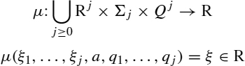
That is, ξ is the cost of the transition δ(a, q1, …, qj) = q when states (q1, …, qj) were reached at costs (ξ1, …, ξj).
Observe that setting j = 0 in the former definition of μ, we have a vector ![]() of initial values associated with the start rules δ(d) for symbols d ∈ Σ0 [i.e., μ(d) = ξ0, d].
of initial values associated with the start rules δ(d) for symbols d ∈ Σ0 [i.e., μ(d) = ξ0, d].
Example 13.3 For the MPP problem, μ can be defined as

The cost function μ can be extended from the transitions Σ to a function ![]() operating on the policies T(Σ):
operating on the policies T(Σ):

As usual, we will not differentiate between μ and ![]() .
.
Definition 13.10 The tree automaton with costs Π = (M, μ) represents the optimization problem (f, S):
min f (x) subject to x ∈ S
if and only if it satisfies
S = L(M) and f (t) = μ(t) for all t ∈ S
Definition 13.11 The optimal value G(q) for a state q is defined as the optimal value of any tree policy t ∈ T(Σ) such that δ(t) = q:
With this definition it is now possible to generalize the dynamic programming equations established in Equation 13.4:
When we instantiate the former equation for the MPP problem we get Equation 13.5. It is now possible to revisit Bellman's optimality principle, stating that any subtree of an optimal tree policy is optimal.
Let us illustrate the set of concepts introduced up to here with a second example: the unrestricted two-dimensional cutting stock problem:
Definition 13.12 The unrestricted two-dimensional cutting stock problem (U2DCSP) targets the cutting of a large rectangle S of dimensions L × W in a set of smaller rectangles using orthogonal guillotine cuts: Any cut must run from one side of the rectangle to the other end and be parallel to one of the other two edges. The rectangles produced must belong to one of a given set of rectangle types ![]() = {T1, …, Tn}, where the ith type Ti has dimensions li × wi. Associated with each type Ti there is a profit ci. No constraints are set on the number of copies of Ti used. The goal is to find a feasible cutting pattern with xi pieces of type Ti maximizing the total profit:
= {T1, …, Tn}, where the ith type Ti has dimensions li × wi. Associated with each type Ti there is a profit ci. No constraints are set on the number of copies of Ti used. The goal is to find a feasible cutting pattern with xi pieces of type Ti maximizing the total profit:

Observe that solutions to the problem can be specified by binary trees. Each node of the tree says whether the cut was vertical (i.e., horizontal composition of the solutions in the two subtrees that we denote by −) or horizontal (i.e., vertical composition of the two existent solutions that will be denoted by |):
Σ = {T1, …, Tn} ∪ {−, |} with ρ(Ti) = 1 ∀ i ∈ {1, …, n} and ρ(|) = ρ(−) = 2
Figure 13.2 presents the solutions α = −(T1, T2), β = |(t1, T2), γ = −(T2, T3), δ = |(T2, T3), −(α, β) = −(−(T1, T2), |(t1, T2)), |(α, β) = |(−(T1, T2), |(t1, T2)), and so on, for some initials rectangles T1, T2, and T3. The labels use postfix notation. Postfix notation provides a more compact representation of the tree. Instead of writing −(α, β), we write the operand and then the operator: α, β−. The tree-feasible solutions will be also called metarectangles.
The set of states is Q = {qx, y/0 ≤ x ≤ L and 0 ≤ y ≤ W}. The idea is that the state qx, y represents a metarectangle of length x and width y. The transition function δ is given by
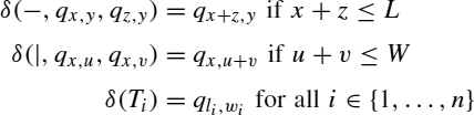
The accepting state is F = {qL, W}. Finally, the cost function is given by
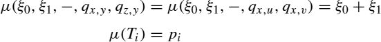

Figure 13.2 Examples of vertical and horizontal metarectangles. Instead of terms, postfix notation is used: α β | and α β − denote the vertical and horizontal constructions of rectangles α and β. Shaded areas represent waste.

Figure 13.3 Calculation of G(qx, y): (a) Sx, y,|; (b) Sx, y−i; (c) Sx, y, i.
When we instantiate Equation 13.8 for this DTFA with costs, we get

where

Figure 13.3 illustrates the meaning of the three parts of the equation.
13.5 PARALLEL ALGORITHMS
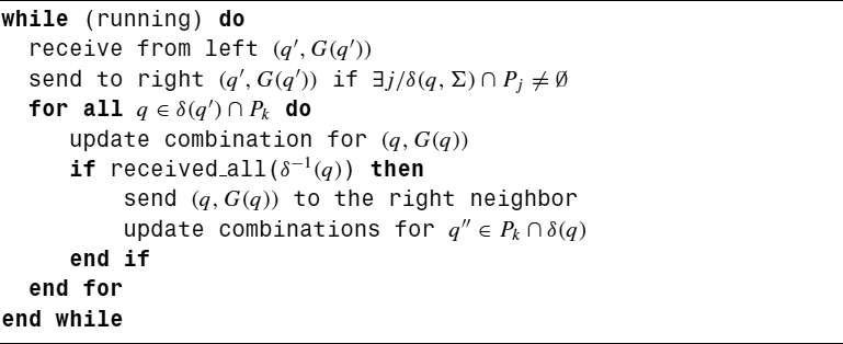
We have again and again successfully exploited the same strategy to get an efficient parallelization of dynamic programming algorithms [6–14]. The DP DAG is partitioned in stages Pk, with k ∈ {1, …, n}, that preserve the complexity order of the DP DAG (Algorithm 13.1). That is: problems/states in stage Pk depend only on subproblems/states on previous stages:

In not a few cases these stages Pk correspond to the levels of the divide-and-conquer search tree shrunk via the equivalence relation defined by Equation 13.2.
On a first high-level description the parallel algorithm uses n processors structured according to a pipeline topology. The processor k executes the algorithm (or an optimized version of it, if it applies) in Figure 13.1. The monadic formalism is used to keep the presentation simple.
Since the number of stages n is usually larger than the number of available processors P, a second, lower-level phase mapping the n processes onto the p processors is required. On homogeneous networks the strategy consists of structuring the p processors on a ring and using a block-cyclic mapping (with block size b). To avoid potential deadlocks on synchronous buffer-limited systems, the last processor is usually connected to the first via a queue process (Figure 13.4). Table 13.1 illustrates the mapping of 12 processes onto a three-processor ring (b = 2). There are two bands. During the first band, processor 0 computes the DP stages P0 and P1. The results of this band produced by processor 2 (i.e., P5) are enqueued for its use by processor 0 during the process of the second band. During such a second band, processor 0 computes P6 and P7.

Figure 13.4 Ring topology (p = 3). The queue process decouples the last and first processors.
TABLE 13.1 Mapping 12 Processes onto a Three-Processor Ring: k = 2
| Processor | Process |
| 0 | (P0, P1) |
| 1 | (P2, P3) |
| 2 | (P4, P5) |
| 0 | (P6, P7) |
| 1 | (P8, P9) |
| 2 | (P10, P11) |
Algorithm 13.1 Pipeline Algorithm for DP: Stage k
The approach presented leads to efficient parallel programs even if the value of b is not tuned. For example, to cite a typical gain for medium and large grain problems, speedups of 8.29 for 16 processors have been reported [5] for the MPP problem on a Cray T3E for an instance of n = 1500 matrices and b = 1.
Finding the optimal value of b for specific DP problems has been the object of study of a number of papers [811–14]. In some cases it is possible to find an analytical formula for the complexity of the parallel algorithm f (input sizes, n, b, p) and from there derive a formula for b that leads to the minimum time [11, 12]. The problem to find the optimal mapping gets more complex when the network is heterogeneous: In such a case, different block sizes bi for i = 0, …, p are considered [13, 14].
13.6 DYNAMIC PROGRAMMING HEURISTICS
Dynamic programming has been extensively used in the land of exact algorithms. Although the search tree is reduced through the equivalence relation formulated in Equation 13.2, the graph is still traversed exhaustively, which usually takes a long time. Even worse, the states are usually elements of a multidimensional space. In the knapsack example, such a space is [0, N − 1] × [0, C], in the MPP, is [1, N] × [1, N], and in the unrestricted two-dimensional cutting stock problem, is [0, L] × [0, W]. More often than not, such a space is prohibitively large, including many dimensions. This is known as the “curse of dimensionality.”5 In the example we consider in this section, the constrained two-dimensional cutting stock problem (C2DCSP or simply 2DCSP), such a space is [0, L] × [0, W] × [0, b1] × [0, b2] × ··· × [0, bN], where bi and N are integers and L and W are the length and width of a rectangular piece of material.
It is in general impossible to keep such huge DP tables in memory for reasonable values of the input parameters. It is, however, feasible, by declining the requirement of exactness, to project the large dimension state space Q = Q1 × ··· × Qn onto a smaller one, Q′ = Q1 × ··· × Qk (with k much smaller than n), producing a projected acyclic graph that can be solved using DP. The solution obtained is an upper bound6 of the optimal solution. In a variant of this strategy, during the combination of the projected DP a heuristic is called that extends the projected solution to a solution for the original DP. In this way we have a heuristic lower bound of the original problem. The two techniques are shown in the following two sections.
13.6.1 Constrained Two-Dimensional Cutting Stock Problem
The constrained two-dimensional cutting stock problem (2DCSP) is an extension of the unconstrained version presented in earlier sections. It targets the cutting of a large rectangle S of dimensions L × W in a set of smaller rectangles using orthogonal guillotine cuts: Any cut must run from one side of the rectangle to the other end and be parallel to one of the other two edges. The rectangles produced must belong to one of a given set of rectangle types ![]() = {T1, …, Tn}, where the ith type Ti has dimensions li × wi. Associated with each type Ti there is a profit ci and a demand constraint bi. The goal is to find a feasible cutting pattern with xi pieces of type Ti maximizing the total profit:
= {T1, …, Tn}, where the ith type Ti has dimensions li × wi. Associated with each type Ti there is a profit ci and a demand constraint bi. The goal is to find a feasible cutting pattern with xi pieces of type Ti maximizing the total profit:

Wang [15] was the first to make the observation that all guillotine cutting patterns can be obtained by means of horizontal and vertical builds of metarectangles, as illustrated in Figure 13.2. Her idea has been exploited by several authors [16–19, 21, 22] to design best-first search ![]() algorithms (see Chapter 12). The algorithm uses the Gilmore and Gomory DP solution presented earlier to build an upper bound.
algorithms (see Chapter 12). The algorithm uses the Gilmore and Gomory DP solution presented earlier to build an upper bound.
13.6.2 Dynamic Programming Heuristic for the 2DCSP
The heuristic mimics the Gilmore and Gomory dynamic programming algorithm [23] but for substituting unbounded ones. feasible suboptimal vertical and horizontal combinations. Let R = (ri)i=1…n and S = (si)i=1…n be sets of feasible solutions using ri ≤ bi and si ≤ bi rectangles of type Ti. The cross product R ⊗ S of R and S is defined as the set of feasible solutions built from R and S without violating the bounding requirements [i.e., R ⊗ S uses (min{ri + si, bi})i=1…n rectangles of type Ti]. The lower bound is given by the value H(L, W), computed as:
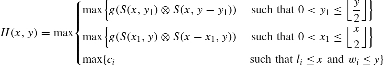
being S(x, y) = S(α, β) ⊗ S(γ, δ) one of the cross sets [either a vertical construction S(x, y0) ⊗ S(x, y − y0) or a horizontal building S(x0, y) ⊗ S(x − x0, y)] where the former maximum is achieved [i.e., H(x, y) = g(S(α, β) ⊗ S(γ, δ))].
13.6.3 New DP Upper Bound for the 2DCSP
The upper bound improves existing upper bounds. It is trivial to prove that it is lower than the upper bounds proposed in refs. 16–19 and 21. The calculus of the new upper bound is made in three steps:
- During the first step, the following bounded knapsack problem is solved using dynamic programming [18, 19]:

for all 0 ≤ α ≤ L × W.
- Then, Fv(x, y) is computed for each rectangle using the equations

where

- Finally, substituting the bound of Gilmore and Gomory [23] by FV in Viswanathan and Bagchi's upper bound [16], the proposed upper bound is obtained:

13.6.4 Experimental Analysis
This section is devoted to a set of experiments that prove the quality of the two DP heuristics presented earlier. The two heuristics are embedded inside the sequential and parallel algorithms presented in Chapter 12. The instances used in ref. 16–19 and 21 are solved by the sequential algorithm in a negligible time. For that reason, the computational study presented has been performed on some selected instances from the ones available in ref. 24. Tests have been run on a cluster of eight HP nodes, each consisting of two Intel Xeons at 3.20 GHz. The compiler used was gcc 3.3.
TABLE 13.2 Lower- and Upper-Bound Results

Table 13.2 presents the results for the sequential runs. The first column shows the exact solution value for each problem instance. The next two columns show the solution value given by the initial lower bound and the time invested in its calculation (all times are in seconds). Note that the designed lower bound highly approximates the final exact solution value. In fact, the exact solution is reached directly in many cases. The last column compares two different upper bounds: the one proposed in ref. 17 and the new upper bound. For each upper bound, the time needed for its initialization, the time invested in finding the exact solution and the number of nodes computed, are presented. Nodes computed are nodes that have been transferred from OPEN to CLIST and combined with all previous CLIST elements. The new upper bound highly improves the previous bound: the number of nodes computed decreases, yielding a decrease in the execution time.
13.7 CONCLUSIONS
A dynamic programming algorithm is obtained simply by adding memoization to a divide-and-conquer algorithm. Automatas and tree automatas with costs provide the tools to model this technique mathematically, allowing the statement of formal properties and general sequential and parallel formulations of the strategy.
The most efficient parallelizations of the technique use a virtual pipeline that is later mapped onto a ring. Optimal mappings have been found for a variety of DP algorithms. Although dynamic programming is classified as an exact technique, it can be the source of inspiration for heuristics: both lower and upper bounds of the original problem.
Acknowledgments
Our thanks to Francisco Almeida, Daniel González, and Luz Marina Moreno; it has been a pleasure to work with them. Their ideas on parallel dynamic programming have been influential in the writing of this chapter.
This work has been supported by the EC (FEDER) and by the Spanish Ministry of Education and Science under the Plan Nacional de I + D + i, contract TIN2005-08818-C04-04. The work of G. Miranda has been developed under grant FPU-AP2004-2290.
REFERENCES
1. L. Wall, T. Christiansen, and R. L. Schwartz. Programming Perl. O'Reilly, Sebastopol, CA, 1996.
2. M. J. Dominus. Higher-Order Perl. Morgan Kaufmann, San Francisco, CA, 2005.
3. C. Rodriguez Leon. Code examples for the chapter “Tools for Tree Searches: Dynamic Programming.” http://nereida.deioc.ull.es/Algorithm-DynamicProgramming-1.02.tar.gz.
4. J. Earley. An efficient context-free parsing algorithm. Communications of the Association for Computing Machinery, 13(2):94–102, 1970.
5. D. Gonzalez Morales, et al. Parallel dynamic programming and automata theory. Parallel Computing, 26:113–134, 2000.
6. D. Gonzalez Morales, et al. Integral knapsack problems: parallel algorithms and their implementations on distributed systems. In Proceedings of the International Conference on Supercomputing, 1995, pp. 218–226.
7. D. Gonzalez Morales, et al. A skeleton for parallel dynamic programming. In Proceedings of Euro-Par, vol. 1685 of Lecture Notes in Computer Science. Springer-Verlag, New York, 1999, pp. 877–887.
8. D. González, F. Almeida, L. M. Moreno, and C. Rodríguez. Pipeline algorithms on MPI: optimal mapping of the path planing problem. In Proceedings of PVM/MPI, vol. 1900 of Lecture Notes in Computer Science. Springer-Verlag, New York, 2000, pp. 104–112.
9. L. M. Moreno, F. Almeida, D. González, and C. Rodríguez. The tuning problem on pipelines. In Proceedings of Euro-Par, vol. 1685 of Lecture Notes in Computer Science. Springer-Verlag, New York, 2001, pp. 117–121.
10. L. M. Moreno, F. Almeida, D. González, and C. Rodríguez. Adaptive execution of pipelines. In Proceedings of PVM/MPI, vol. 2131 of Lecture Notes in Computer Science. Springer-Verlag, New York, 2001, pp. 217–224.
11. F. Almeida, et al. Optimal tiling for the RNA base pairing problem. In Proceedings of SPAA, 2002, pp. 173–182.
12. D. González, F. Almeida, L. M. Moreno, and C. Rodríguez. Towards the automatic optimal mapping of pipeline algorithms. Parallel Computing, 29(2):241–254, 2003.
13. F. Almeida, D. González, L. M. Moreno, and C. Rodríguez. Pipelines on heterogeneous systems: models and tools. Concurrency—Practice and Experience, 17(9):1173–1195, 2005.
14. F. Almeida, D. González, and L. M. Moreno. The master–slave paradigm on heterogeneous systems: a dynamic programming approach for the optimal mapping. Journal of Systems Architecture, 52(2):105–116, 2006.
15. P. Y. Wang. Two algorithms for constrained two-dimensional cutting stock problems. Operations Research, 31(3):573–586, 1983.
16. K. V. Viswanathan, and A. Bagchi. Best-first search methods for constrained two-dimensional cutting stock problems. Operations Research, 41(4):768–776, 1993.
17. M. Hifi. An improvement of Viswanathan and Bagchi's exact algorithm for constrained two-dimensional cutting stock. Computer Operations Research, 24(8): 727–736, 1997.
18. S. Tschoke, and N. Holthöfer. A new parallel approach to the constrained two-dimensional cutting stock problem. In A. Ferreira and J. Rolim, eds., Parallel Algorithms for Irregularly Structured Problems. Springer-Verlag, New York, 1995. http://www.uni-paderborn.de/fachbereich/AG/monien/index.html.
19. V. D. Cung, M. Hifi, and B. Le-Cun. Constrained two-dimensional cutting stock problems: a best-first branch-and-bound algorithm. Technical Report 97/020. Laboratoire PRiSM–CNRS URA 1525, Université de Versailles, France, Nov. 1997.
20. G. Miranda and C. León. OpenMP parallelizations of Viswanathan and Bagchi's algorithm for the two-dimensional cutting stock problem. Parallel Computing 2005, NIC Series, vol. 33, 2005, pp. 285–292.
21. L. García, C. León, G. Miranda, and C. Rodríguez. A parallel algorithm for the two-dimensional cutting stock problem. In Proceedings of Euro-Par, vol. 4128 of Lecture Notes in Computer Science. Springer-Verlag, New York, 2006, pp. 821–830.
22. L. García, C. León, G. Miranda, and C. Rodríguez. two-dimensional cutting stock problem: shared memory parallelizations. In Proceedings of the 5th International Symposium on Parallel Computing in Electrical Engineering. IEEE Computer Society Press, Los Alamitos, CA, 2006, pp. 438–443.
23. P. C. Gilmore and R. E. Gomory. The theory and computation of knapsack functions. Operations Research, 14:1045–1074, Mar. 1966.
24. DEIS Operations Research Group. Library of instances: two-constraint bin packing problem. http://www.or.deis.unibo.it/research_pages/ORinstances/2CBP.html.
1The word attributes refers here to the information saved in the nodes. In the former 0–1 knapsack problem example, the attributes were the pair (k, c) holding the object and the capacity.
2But not always; DP is not limited to optimization problems and has almost the same scope as DnC. As an example, the early parsing algorithm uses dynamic programming to parse any context-free language in O(n3) time [4]. Hardly parsing can be considered an optimization problem.
3Notice that j can be zero, and therefore transitions of the form δ(b) = q, where b ∈ Σ0, are allowed.
4The notation ![]() for trees t, t′ ∈ T(Σ ∪ Q), means that a subtree a(q1, …, qk) ∈ Q inside t has been substituted for by q = δ(a, q1, …, qk). The notation
for trees t, t′ ∈ T(Σ ∪ Q), means that a subtree a(q1, …, qk) ∈ Q inside t has been substituted for by q = δ(a, q1, …, qk). The notation ![]() is used to indicate that several one-step substitutions
is used to indicate that several one-step substitutions ![]() have been applied.
have been applied.
5A term coined by Richard Bellman, founder of the dynamic programming technique.
Optimization Techniques for Solving Complex Problems, Edited by Enrique Alba, Christian Blum, Pedro Isasi, Coromoto León, and Juan Antonio Gómez
Copyright © 2009 John Wiley & Sons, Inc.