C H A P T E R  12

Data Profiling and Scrubbing

Code, load, and explode.

—Steve Hitchman

Projects that require bringing together data from multiple sources—for example, data warehouse, data mart, or operational data store (ODS) projects— are extremely common. You could spend months gathering business requirements, putting together technical specifications, designing target databases, and coding and testing your ETL process. You could spend an eternity in “ad hoc maintenance mode” rewriting large sections of code that don’t handle unanticipated bad or nonconforming data. This scenario is the result of a failure to properly plan and execute data integration projects—a phenomenon known as code, load, and explode.

Anytime you need to bring together data from two or more systems, you have a data integration project on your hands. Proper data integration requires a lot of grunt work. Unfortunately, it’s one of the least exciting and glamorous parts of any project—thorough planning and process formalization, investigation of source systems, interrogation of source data, generation of large amounts of documentation . By accident or by choice, the scope of data integration requirements and the cost of not doing it right are often underestimated in enterprise projects. Data integration requires a lot of generally low-profile analysis, but failure to do it properly can result in high-profile project failures. This chapter shows how SSIS can help you properly profile and cleanse your data.

Data Profiling

Data profiling, at its core, is the process of gathering statistical information about your data. The purpose is to ensure that your source data meets your expectations by answering questions such as the following:

Does my source data contain nulls? You may expect certain source data columns to contain no nulls, or to contain a certain number of nulls (fewer than 10 percent, for instance). Profiling your source data will reveal whether the number of nulls meets your expectations.

Does my source data contain all valid values? This involves defining domains, or sets of valid values, for your source data. As examples, you might expect a Gender column to contain only Male or Female values, or you might expect a Price column to contain only positive numeric values between 0.01 and 500.00. Profiling will tell you whether your source data falls within its expected domains.

Does the distribution of my data fit my expectations? Answering this question requires industry- and business-specific domain knowledge. For instance, you might expect most of the prices for items in your inventory to fall between $20 and $50. An analysis of your data might show that the majority of items in inventory are actually priced lower than $20, which could point to either (1) a bad initial assumption about the business, or (2) a data quality problem.

How does my source data align with data from other systems? Consider reference data such as US state codes. Several types of codes could be used by any given source system: two-character Postal Service codes such as AL, DE, and NY; two-digit FIPS (Federal Information Processing Standard) numeric codes such as 01, 02, 03; or even integer surrogate keys. Answering this question will let you recognize differences in key attributes and align the values in key attributes.

What are my business keys? Successful data integration projects, such as BI projects, require identification of business keys in your source data. Data warehouse updates and data mart slowly changing dimension (SCD) processing depend on knowledge of your source data business keys.

Answering these questions might require profiling single columns or sets of columns. As an example, most industrialized countries implement postal code systems to facilitate mail delivery. The format and valid characters in postal codes vary from country to country. Postal codes in the United States (also known as Zone Improvement Plan, or ZIP, codes) consist of either five or nine numeric digits, such as90071 or 10104-0899. In Canada, postal codes consist of six alphanumeric characters—for example, K1P 1J9. You may need to profile country names and postal codes from your source data in combination with one another to validate proper postal code formats.

In addition to answering questions about the quality and consistency of your source data, you may also isolate information about the relationships in your source databases. One thing that many legacy source databases seem to have in common is a lack of referential integrity and check constraints. Throw in an utter lack of documentation, and these source systems present themselves as complex puzzles, often requiring you to establish relationships between tables yourself.

Data Profiling Task

The Data Profiling task is a useful way to grab statistical information about your source data. Much of the major functionality is comparable in many respects to other data-profiling software packages available on the market. The Data Profiling task grabs the specified source data, analyzes it based on the criteria you specify, and outputs the results to an XML file. The Data Profiling task is shown in Figure 12-1.

Figure 12-1. Data Profiling task in a package control flow

The Data Profiling task requires a File Connection Manager pointing to the XML file you want it to create or overwrite. We configured our File Connection Manager to point at a file named C:SampleDataProfileOutput.xml, as shown in Figure 12-2.

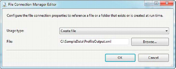
Figure 12-2. Configuring the File Connection Manager to point at an XML output file

One drawback of the Data Profiling task is that it is limited to data that can be retrieved via an ADO.NET Connection Manager. The Data Profiling task requires a connection to SQL Server and uses the SqlClient Data Provider, shown by the ADO.NET Connection Manager Editor in Figure 12-3.

Figure 12-3. Connection Manager editor providers

The General page of the Data Profiling Task Editor lets you choose destination options including the destination type, the destination connection manager, whether the destination should be overwritten if it exists already, and the source time-out (in seconds). Figure 12-4 shows the editor’s General page.

Figure 12-4. General page of the Data Profiling Task Editor

On the Profile Requests page, you can choose and configure profile requests, each representing a specific type of analysis to perform and a set of statistics to collect about your source data. Figure 12-5 shows many of the types of profile requests that can be selected. Table 12-1 describes the profile requests you can choose. You’ll look at configuring individual data profile requests in the following sections.

Figure 12-5. Profile Requests page of the Data Profiling Task Editor

Data Profile Viewer

After the Data Profiling task generates an XML output file, you can view the results by using a tool called the Data Profile Viewer, which is found in the SQL Server Integration Services folder on the Windows Start menu. Figure 12-6 shows the Data Profile Viewer on the Start menu.

Figure 12-6. Data Profile Viewer on the Start menu

After you launch the Data Profile Viewer, you can open the XML file generated by the Data Profiling task by clicking the Open button and selecting the file, as shown in Figure 12-7.

Figure 12-7. Opening the Data Profiling task output in the Data Profile Viewer

After you open the Data Profiling task output file in the Data Profile Viewer, you’ll see a list of all the profile requests you selected on the left side of the window. Clicking one of the profile requests displays the details on the right side of the window. You can click the detail rows on the right side to show even more detail. In Figure 12-8, we’ve selected the Candidate Key profile request and drilled into the details of the EventId column.

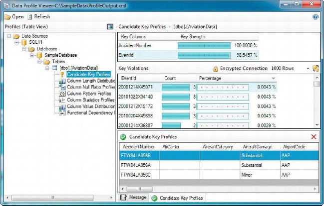
Figure 12-8. Viewing the results of a Data Profiling task Candidate Key profile request

Column Length Distribution Profile

The Column Length Distribution profile reports the distinct lengths of string values in the columns you select, and the percent of rows in the table that each length represents. As an example, US ZIP codes must be five to ten characters in length (ZIP+4, including the hyphen); any other string length for these data values may be considered invalid. When analyzing your data, you may find that some of your ZIP codes are the wrong length. After choosing the Column Length Distribution profile request, you can configure it as shown in Figure 12-9.

Figure 12-9. Configuring the Column Length Distribution profile request

For the Column Length Distribution profile request, you need to configure the source connection manager and choose the table and columns you wish to profile. Choosing wildcard (*) as the column indicates that you want to use all the columns in the table (nonstring columns are ignored). You can also choose to ignore leading or trailing spaces in your data.

After you run the Data Profiling task, the Column Length Distribution profile request generates a list of string-value columns. Selecting one of these columns shows you the distribution of string data lengths in that column. Clicking one of the lengths in the Length Distribution list shows the details, listing the values that match that length.

In Figure 12-10, we’ve selected the AccidentNumber column, which has data in three lengths: 9 characters, 10 characters, and 11 characters. We then drilled into the 9-character values to see the rows containing these values. After viewing the column-length distributions, we can see that the AccidentNumber column generally holds 10-character lengths. The small percentage of 9-character and 11-character values may represent a data quality issue with the source data.

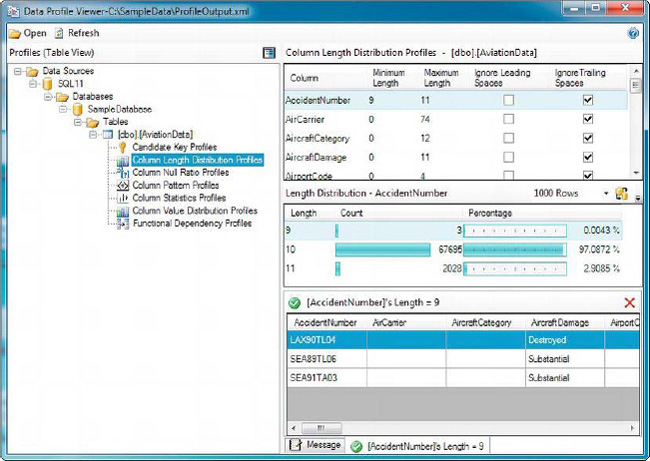
Figure 12-10. Reviewing details of the Column Length Distribution profile

Column Null Ratio Profile

The Column Null Ratio profile helps you identify columns that contain more (or fewer) nulls than expected. If you have a column for which you expect very few nulls, but discover a very large number of nulls, it could indicate a data quality issue (or it may mean that the assumptions about your data need to be changed). The Column Null Ratio profile is simple to configure. Like the Column Length Distribution profile request, you must choose an ADO.NET Connection Manager, a table or view, and the column you want to profile. Like the Column Null Ratio profile request, the Column Null Ratio request lets you choose (*) to profile all columns. In Figure 12-11, we’ve chosen to profile all columns in the AviationData table.

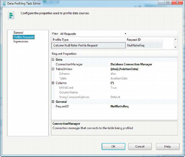
Figure 12-11. Configuring the Column Null Ratio profile request

The results can be viewed in the Data Profile Viewer. In our example, we’ve focused on the AircraftDamage column, which contains no nulls, as shown in Figure 12-12.

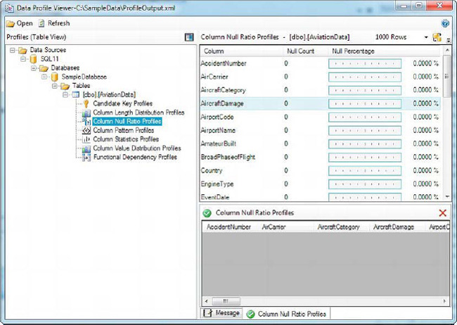
Figure 12-12. Reviewing the results of the Column Null Ratio profile

Column Pattern Profile

The Column Pattern profile is useful for identifying patterns in string data, such as postal codes that aren’t formatted according to the standards for a given country. This profile returns regular expression patterns that match your string data, which can make it easy to identify string data that does not fit expected patterns. As an example, a US five-digit ZIP code should fit the regular expression pattern d{5}”, which represents a string of exactly five numeric digits. Any five-digit US ZIP codes that do not match this pattern are invalid.

Like the other profile requests, the Column Pattern profile request requires an ADO.NET Connection Manager, a table or view, and a source column. In addition, the Column Pattern profile request has many more options available than the other profile requests we’ve covered so far. The following options allow you to refine your Column Pattern profile request:

MaxNumberOfPatterns: The maximum number of patterns that you want the Data Profiling task to compute. The default is 10, and the maximum value is 99.

PercentageDataCoverageDesired: The percentage of rows to sample when computing patterns. The default is 95.

CaseSensitive: A flag indicating whether the generated patterns should be case-sensitive. The default is False.

During the process of computing patterns to fit your string data, the Data Profiling task tokenizes your strings (breaks them into individual “words” or substrings). Two options are included for controlling this tokenization behavior:

Delimiters: This is a list of characters that are treated as spaces when tokenizing strings. By default, the delimiters are the space, the tab ( ), carriage return (“ ”), and newline (“ ”).

Symbols: The list of symbols to keep when tokenizing data. By default, this list includes the following characters: ,.;:-"'`~=&/@!?()<>[]{}|#*^%.

The Column Pattern profile request also allows you to tag, or group, tokens. Tags are stored in a database table with two-character data columns named Tag and Term. The Tag column holds the name of the token group, and the Term column holds the individual tokens that belong to the group. For performance reasons, it’s recommended that if you use this option, use 10 tags or fewer and no more than 100 terms per tag. The following options control the tagging behavior:

TagTableConnectionManager: An ADO.NET Connection Manager using the SqlClient provider to connect to a SQL Server database.

TagTableName: The name of the table holding the tags and terms. Must have two columns named Tag and Term.

Figure 12-13 shows how we configured the Column Pattern profile request for our sample.

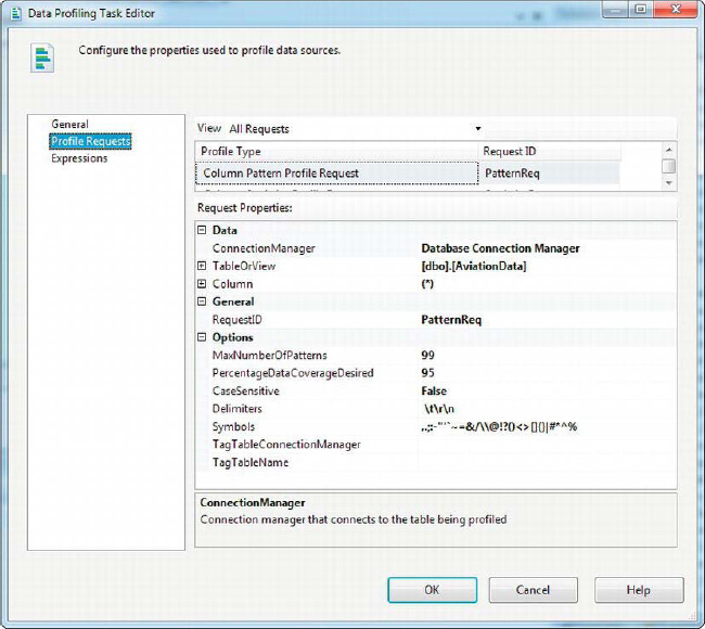
Figure 12-13. Configuring the Column Pattern profile request

The results of the Column Pattern profile are shown in Figure 12-14. We focused on the EventYear column and found that all data matched the pattern dddd, which is the expected pattern of four numeric characters in a row. Because all of the string values in this column match the valid pattern, we are a little closer to confirming that the values are valid.

Figure 12-14. Reviewing the Column Pattern profile results

Column Statistics Profile

The Column Statistics profile helps to quickly assess data that is outside of the normal range, or tolerances, for a given column. You might find that your column contains dates of birth that are in the future, for example. You can also use the basic statistical information provided to determine whether your data fits the statistical normal distribution.

Configuring the Column Statistics profile request is similar to the previously described profile requests. You need to choose a connection manager, table or view, and a source column. As before, you can you can use (*) to profile all columns. We configured our Column Statistics profile request to use the AviationData table, as shown in Figure 12-15.

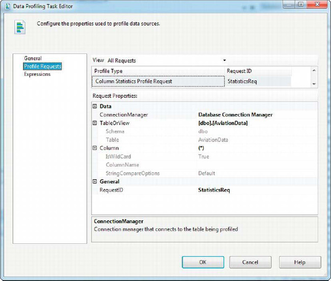
Figure 12-15. Configuring the Column Statistics profile request

The Column Statistics profile will profile columns that hold date/time and numeric data, such as DATETIME, INT, FLOAT, and DECIMAL columns, for example. For date/time data, the profile calculates the minimum and maximum; for numeric data, it calculates the minimum, maximum, mean (average), and standard deviation. Results of our sample Column Statistics profile are shown in Figure 12-16.

Figure 12-16. Reviewing the results of the Column Statistics profile request

Column Value Distribution Profile

The Column Value Distribution profile reports all the distinct values in a column and the percentage of rows in the table that each value represents. You can use this information to determine whether different values occur with the expected frequency. You may find, for instance, that a column’s default value occurs far more often than you anticipated.

The Column Value Distribution profile request has several options to configure. The usual suspects are here: you need to configure an ADO.NET Connection Manager, choose the source table or view, and select the column to profile. You also need to choose a ValueDistributionOption: FrequentValues (the default) limits the results reported to those that meet or exceed a given threshold, and AllValues reports all the results regardless of how many times they occur. The FrequentValueThreshold option is a numeric value—the minimum threshold used to limit the results returned when the FrequentValues option is selected. Figure 12-17 shows how we configured the Column Value Distribution profile request by using the AllValues options.

Figure 12-17. Configuring the Column Value Distribution profile request

The results of profiling the columns of the AviationData table are shown in Figure 12-18. The column displayed is the State column, with occurrence counts and occurrence percentages shown.

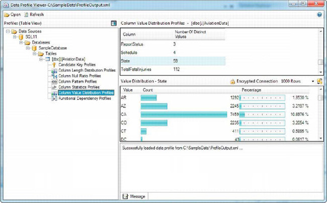
Figure 12-18. Results of Column Value Distribution profile of the State column

Candidate Key Profile

The Candidate Key profile profiles one or more columns to determine the likelihood that a column (or set of columns) would be a good key, or approximate key, for your table. The Candidate Key profile is a useful tool when you are trying to identify your business keys (attributes that uniquely identify business transactions or objects).

As with the other profile requests, you must configure the Candidate Key profile with an ADO.NET Connection Manager, a source table or view, and columns. Unlike the other profile requests, in which you choose only a single column or all columns by using the wildcard (*), this profile request allows you to choose many columns. This makes sense because a given candidate key can consist of multiple columns, and you may want to test several permutations of column sets for viability as candidate keys. The drop-down menu for choosing KeyColumns is shown in Figure 12-19. You can choose one or more columns in several combinations, such as the following:

Single named column: If you choose a single column, it will be tested for usefulness as a candidate key.

Multiple named columns: If you choose multiple named columns, they are all tested together for usability as a composite candidate key. For instance, if you choose the AirCarrier, AircraftCategory, EventDate, and State columns, the Data Profiling task will test all of the columns together for usability as a single candidate key.

Single wildcard: If you choose the wildcard (*) as your column, the Data Profiling task profiles every column in your table, testing each individually for usability as a candidate key.

Single wildcard and named columns: If you choose the wildcard (*) and one or more named columns, the Data Profiling task will test combinations of the named columns and the other columns in the table for candidate key viability. As an example, you might choose AirportCode and (*) in your profile request, in which case the Data Profiling task will test the AirportCode column in combination with every other column in the table.

Multiple wildcards: If you choose multiple wildcard (*) columns, the Data Profiling task tests the permutations of the specified number of column combinations for usability as candidate keys. For instance, if you choose two wildcards, the task profiles all combinations of two columns in your table for uniqueness.

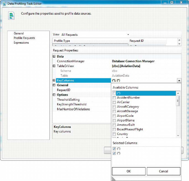
Figure 12-19. Data Profiling Task Editor

Figure 12-20 demonstrates the Candidate Key profile output. The strength of the proposed key columns AirCarrier, AircraftCategory, EventDate, and State are approximately 87 percent unique. The output goes even further and shows the duplicate rows for each of the key violations as well as the count of the infractions.

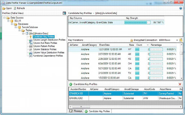
Figure 12-20. Tolerances for candidate keys

Functional Dependency Profile

The Functional Dependency profile allows you to use the profiling task to find dependencies on the table. The dependencies test to see how the values in the specified columns determine the values of the dependent columns. Using the (*) as the DeterminantColumns property allows us to test every column as the determinant of all the combinations allowed by the DependentColumns. The (*) value in the DependentColumn property allows us to test every combination of the columns in the table to be dependent on the specified determinant. Using the (*) notation for both properties will pit each column against every combination of all the columns for a dependency report. The 0.95 threshold indicates that only 95 percent or better will define a useful data dependency, as displayed in Figure 12-21.

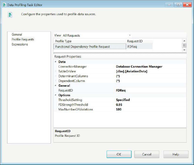
Figure 12-21. Functional Dependency profile request

Figure 12-22 demonstrates the results of the Functional Dependency profile request. The report shows you the overall strength of each of the tests as well as the different violations. The tab below the report shows the individual data elements that were used for profiling the dependency and their strengths.

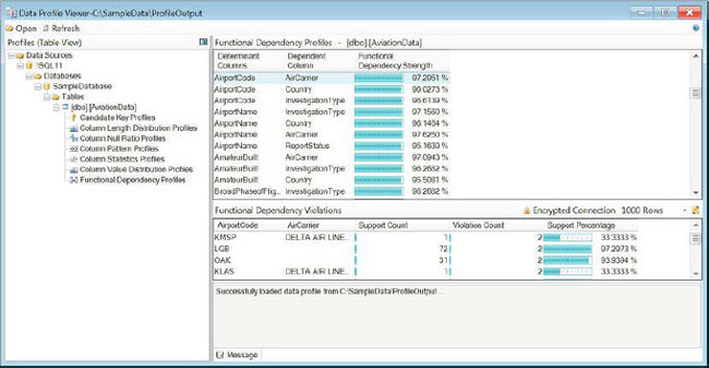
Figure 12-22. Functional Dependency profile output

Fuzzy Searching

One of the risks of adding new data to any set is the possibility of unclean, or nonconforming, data entering the system. This usually comes in the form of violating the rules of a character column’s domain—for example, alphabet characters for a US ZIP code column being entered. SSIS provides two data flow transformations to clean up the data inconsistencies: the Fuzzy Lookup and the Fuzzy Grouping. They both utilize a token-based approach to determine matches between incoming data and the reference data. After the matches are successfully completed, you can replace the old data with the new conforming data.

Fuzzy Lookup

The Fuzzy Lookup returns close matches of reference data for the incoming data stream. This is in contrast to the Lookup transformation, which returns exact matches. One of the advantages to using the Fuzzy Lookup is its ability to return data that contains the strings stored in the lookup table. The lookup table in this instance would be representative of clean data. The Fuzzy Lookup task can be used to allow only data with acceptable matches to be passed through.

For this example, we are using our dbo.State table as the source of data. We set a list of lookups to isolate the states that match any members of the list. The code in Listing 12-1 demonstrates the table structures and the lookup list.

The dbo.StateFuzzyMatch table contains all the key words that we will be searching for in the State data. We inserted some keywords that we need to find in the Fact attribute of the dbo.State data. We will store the successful matches of the Fuzzy Lookup operation in dbo.StateFuzzyLookup. This table includes additional columns that include the fuzzy match details, including the following:

FuzzyMatchData is the element in the lookup table that matched the incoming data.

_Similarity represents the level of similarity between the incoming data and the lookup element. This value can be used to adjust the similarity threshold on the Fuzzy Lookup component to eliminate unwanted matches. This alias can be modified for each of the separate columns handled in the fuzzy matching.

_Confidence represents the confidence of the match. Previous versions of SSIS have taken into account the best similarity and the number of positive matches for a given data row to calculate this value.

Performing a Fuzzy Lookup and limiting the data to only rows that successfully match will result in the data shown in Figure 12-23. Listing 12-2 shows the query that will retrieve the positive matches and the statistics of the operation. As the results of the query demonstrate, a direct correlation between similarity and confidence does not necessarily exist for the matches in this dataset.

Figure 12-23. Fuzzy Lookup matches

Having seen the output and the SQL Server table set up, let us tie back to the SSIS package development that is required for implementing the Fuzzy Lookup. The Fuzzy Lookup is a Data Flow task component and requires a data stream for the matching. The OLE DB source we utilize contains the query in Listing 12-3 to extract all the data that we have on the states that make up the United States of America.

At the onset of development, our requirement was to isolate states whose fact contained some very specific tokens. We loaded these tokens in dbo.StateFuzzyMatch. Unlike the Lookup component, which can use a query to create the lookup list, the Fuzzy Lookup must point to the table in order to perform its matches. The component creates indexes on the table in order to expedite the match operations. Figure 12-24 demonstrates the options we used for the Fuzzy Lookup. We did not choose to save the index but instead allow the component to regenerate a new index at each execution. The index used for that execution is not saved. For static tables, it is recommended that the index is saved.

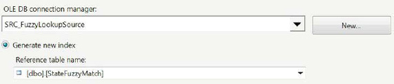
Figure 12-24. FZL_MatchFact—Reference table configuration

After the table is specified for the component, you can select the column mapping for the lookup matching, as shown in Figure 12-25. If you are required to do matches on multiple columns, you can perform the matches here. The editor draws lines to easily identify the mappings between the input columns and the lookup columns. In our sample, the match is performed on one column, but just like the Lookup component, the Fuzzy Lookup component can utilize multiple columns for its matching criteria.

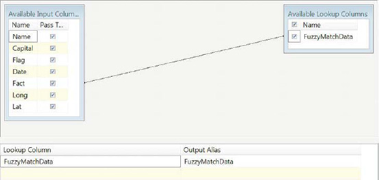
Figure 12-25. FZL_MatchFact—Columns

The Create Relationships Editor, shown in Figure 12-26, allows you to specify the criteria for each of the mappings involved in the lookup. To open this editor, you have to right-click on the background of the Columns mapping area and select Edit Mappings. The key fields in this editor are Mapping Type, Comparison Flags, and Minimum Similarity. The options for Mapping Type are Fuzzy and Exact. Selecting Exact is the same as forcing Lookup component restrictions on the Fuzzy Lookup. It will forcibly change the Minimum Similarity to be 1, a 100 percent match. The Comparison Flags allow flexibility in terms of how the matches are performed. In our example, we were concerned with ignoring only the case of the characters of the data. The Minimum Similarity sets the threshold for the match to be successful for each of the relationships. The Similarity Output Alias allows you to store the similarity information for each relationship. In our example, we are storing only the overall similarity of the lookup. Because it is a one-column match, the similarity matches the relationship similarity. Just like the Lookup component, the lookup column can be added to the pipeline and sent to the destination. The editor allows you to alias the lookup column if you need to add it to the pipeline.

Figure 12-26. FZL_MatchFact Create Relationships

The Advanced tab of the Fuzzy Lookup Editor, shown in Figure 12-27, allows you to define the delimiters and the overall similarity threshold for each of the matches. The option that allows you to define the maximum number of matches will duplicate data rows for each successful match. For this example, we are using only whitespaces as delimiters for the tokens. By default, a few punctuation characters are defined as delimiters.

Figure 12-27. FZL_MatchFact—Advanced

The entire Data Flow task is shown in Figure 12-28. The Fuzzy Lookup component has a warning message because the sizes of the Fact column and the FuzzyMatchData column do not match. We added the Conditional Split component so that only rows with matching data pass through to the table. The FuzzyMatch output uses !ISNULL(FuzzyMatchData) as the splitting condition.

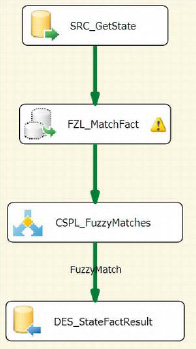
Figure 12-28. DFT_FuzzyLookupSample

Fuzzy Grouping

The Fuzzy Grouping component attempts to reduce the number of duplicates within a dataset based on the match criteria. The component will accept only the string data types, Unicode and Code page, to perform the matching operations. The transformation itself will create temporary tables and indexes on the server in order to perform the matching operations efficiently. For this example, we will use the same source component that we used for the Fuzzy Lookup example. The configuration of the Fuzzy Grouping transformation is very similar to Fuzzy Lookup in that it allows you to choose the Match Type, the Minimum Similarity, Comparison Flags, and other options as well. In addition, Fuzzy Grouping allows you to specify whether data may contain numeric characters by providing the Numerals option. The Numerals option enables you to perform better matches on alphanumeric information for which the numeric data poses significant implications at the beginning or end of the string. This option becomes useful for street address information or alphanumeric postal codes. For our example of Fuzzy Grouping, we will utilize the table shown in Listing 12-4 as the destination table for the results of the match.

The Fuzzy Grouping transformation adds a few columns to the pipeline in order to track the grouping. Some of the columns track the statistics behind the grouping, while others trace the records as they come through the pipeline:

_key_in traces the original record as it comes through the Data Flow task. This column is for all intents and purposes an identity column. Every row in the dataset receives its own unique value.

_key_out connects a grouped row to the _key_in value of the matching row that it most closely resembles.

_score displays the similarity between the row and the matching row.

Fact_clean represents the matching row’s value for the Fact column.

_Similarity_Fact shows the similarity between the Fact column of the row and the matching row’s Fact value.

Listing 12-5 shows how the grouping matched the states based on the facts recorded about them. The join conditions in the first query show how the columns added by the Fuzzy Grouping allow you to trace back the data to their original form. The second query allows you to replace the state’s original fact with the fact that the Fuzzy Grouping transformation calculated to be the closest.

Figures 12-29 and 12-30 demonstrate the results of the queries shown in Listing 12-5. You may even be able to determine the tokens used to determine the matches just by looking at Figure 12-28. For example, for Colorado and Louisiana, the tokens used for the matching were most likely the only state.  As for Arizona and Montana, National Park was the most likely candidate. The scores for these matches are relatively low because we set the similarity threshold to 0.08. The facts that match are usually shorter strings matching to longer strings that contain a significant number of the tokens.

Figure 12-29. Fuzzy Grouping results

The result set shown here simply demonstrates how the matched data is used rather than the original values. This transformation can provide some useful insight when attempting to initiate a data cleansing project. Business names, addresses, and other contact information can be easily consolidated with the proper use of this component. The value of the Fuzzy Grouping transformation begins to show itself when the data starts following a standardized set.

Figure 12-30. Fuzzy Grouping data replaced

Data Previews

One of the most useful features of SSIS is the ability to see the data as it flows through the Data Flow task. There are a few options that allow you to sample the data. Data Viewers allow you to see the data in various forms between two different components of the Data Flow task. The Row Sampling and Percentage Sampling transformations allow you to extract sample data directly from the dataset.

Data Viewer

The Data Viewer option allows you to get a quick snapshot of your data stream as it moves through your Data Flow task. The viewers can be enabled between any two components within your Data Flow task. Figure 12-31 demonstrates how the Data Viewer is defined on a Data Flow task. In order to enable a Data Viewer, you have to right-click a connector between two components and select Enable Data Viewer.

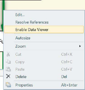
Figure 12-31. Enabling the Data Viewer

After the Data Viewer has been enabled, a small icon will appear on the connector you chose. The icon is a small magnifying glass indicating an in-depth look at the pipeline at a singular point in time. Figure 12-32 demonstrates a connector with a Data Viewer enabled. The Data Viewer can greatly assist you during development because it can allow you to look at data without having to commit it to a table or an object variable. One of the areas this object helps in data profiling is during data conversions. Suppose your Data Conversion transformation is failing without very specific error messages. The Data Viewer can help you identify the rows that are causing the error, allowing you to initiate actions to either fix the bad data or to ignore it. The Data Viewer can also be utilized to gauge the success of Lookup components or Merge Join transformations.

Figure 12-32. Enabled Data Viewer

The Data Viewer shows the data during runtime. The data is shown buffer by buffer as it passes through the connector between two components. There are options on how to display the data, the most popular being the grid. The grid displays the data in a tabular format with the ability to copy the data to the clipboard for later use. The grid appears in a separate window during the Debug mode of Visual Studio. Figure 12-33 shows the Data Viewer after a Fuzzy Lookup component.

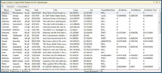
Figure 12-33. Data Viewer of Fuzzy Lookup output

The name of the window helps identify its placement in the package. In this case, the Data Viewer is enabled after a Fuzzy Lookup component, and therefore the window’s derived name is Fuzzy Lookup Output Data Viewer at DFT_DataViewer. The window also contains a green arrow button that informs Visual Studio to proceed with the execution of the package and allow the data rows to pass through the connector. The Detach button will preserve the window and allow the package to proceed with its execution. The Copy Data button will copy highlighted rows and the column headers of the dataset to the clipboard. Clicking a particular column header will automatically sort the data according to the values in that particular buffer. Closing the Data Viewer window will also force the Visual Studio debugger to continue the execution of the package.

Data Sampling

The SSIS Data Flow task has some useful components that assist in viewing random data samples during runtime. These components are the Row Sampling and Percentage Sampling transformations. These transformations will extract the defined sampling of rows from the data stream as it passes through. Without a Sort transformation or ORDER BY clause, the data should be in random order as it passes through. The sampling transformations will reflect this by selecting a random sample set from the data. The alternative to the sampling transformations is the TOP N recordset from SQL Server. The main difference is that SSIS will attempt a truly random set, whereas TOP N will return that number or percentage of records as they are read from disk.

Row Sampling

The Row Sampling transformation allows you to define the number of rows that you would like to extract from the data stream as your sample set. This sample set is completely removed from the pipeline. The data is randomly selected unless you select a seed. If you specify a seed, you will use it in the random-number generation when selecting the rows for your row sample. Figure 12-34 demonstrates a Data Flow task utilizing a Row Sampling component.

Figure 12-34. Row Sampling example

The destinations for the datasets are recordet destinations. We used object data type variables to store each of the outputs. The Row Sampling transformation was configured to use only 10 rows from the dataset as the sample set. The rest of the rows were to be ignored for the sampling exercise. In execution results, you can see that the Sampling Selected Output completely removed the rows from the original pipeline and created as a separate stream, Sampling Unselected Output. In this functionality, the Row Sampling transformation works similarly to the Conditional Split transformation. The Conditional Split transformation may also be used to extract a sample from your dataset by using a condition that will randomly change between True and False for certain rows. The main challenge would be defining the size of the sample set.

Percentage Sampling

The Percentage Sampling transformation works similarly to the Row Sampling transformation. Instead of relying on a predefined number of rows, the Percentage Sampling transformation relies on a required percentage of the dataset to be used as the sample set. Figure 12-35 demonstrates a Data Flow task utilizing a Percentage Sampling transformation to extract a sample dataset.

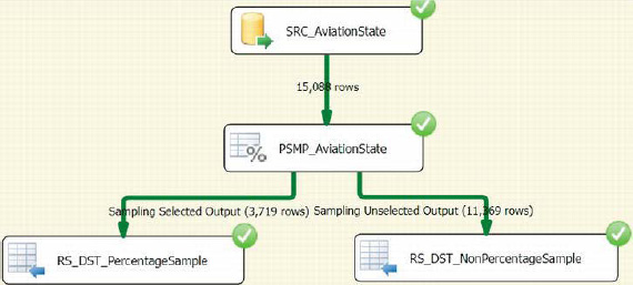
Figure 12-35. Percentage Sampling example

For this example, we configured the Percentage Sampling transformation to select 25 percent of the rows from the dataset as the sample set. The initial row count from the source is 15,088. The 3,719 rows are approximately 24.64 percent of 15,088 rows; 25 percent would have been 3,722 rows. The Percentage Sampling transformation does not provide exact percentage breaks when it comes to sampling the rows, but it comes very close. After executing the Data Flow task several times, you will realize that the number of records is not always consistent. The number will be around the percentage specified but will not necessarily be exact.

Summary

Data integration projects require a lot of overheard to synchronize the data from various systems. SSIS provides various tools to analyze this data so that a well-informed plan can be formalized. These tools include the Data Profiling task, Fuzzy search transformations, data sampling transformations, and viewers to analyze data that traverses your data flow. Using these built-in tools enables you to get a snapshot of the data’s state very quickly. The next chapter covers the logging and auditing options available to you as you extract, transform, and load your data from various systems into potentially different systems.