C H A P T E R 14
Heterogeneous Sources and Destinations
We want to further eliminate friction among heterogeneous architectures and applications without compromising their distinctive underlying capabilities.
—Microsoft cofounder Bill Gates
One of the key elements of a data integration tool is the ability to handle disparate sources and destinations. SQL Server Integration Services 2011 allows you to extract from any storage method and load data into just as many data storage systems. The toolset provided by Integration Services truly attempts to achieve the goal outlined by Bill Gates to allow various systems to mesh well together. As discussed in previous chapters, data integrity is a key element to success of integration projects, and SSIS provides transformations and components that allow you to handle the nonconforming data.
Data storage comes in various forms. This includes text files that cannot inherently enforce data quality (such as data types or foreign keys), other RDBMSs (including Oracle or DB2), XML files, web services, or even the Active Directory. All these systems can hold data in some structure that SSIS can unravel and integrate into one system. However, the destination is not limited to just SQL Server. Data can be loaded back into an original form if the requirements specify such a need.
This chapter covers some of the sources and destinations that SSIS can access. This chapter relies heavily on the information provided in Chapter 4 for its basis and then builds upon that foundation to provide you with examples that you can use in your everyday process.
SQL Server Sources and Destinations
The easiest of all sources and destinations for SSIS to handle is SQL Server. Reading from prior versions is relatively easy, but loading into a prior version may require some data conversions to handle newer or deprecated data types. As we mentioned in Chapter 4, the most efficient way to extract data from a SQL Server database is by using the SQL command option to write your own SQL statement. This is the recommended option to use on a SQL Server source component for several reasons. The first and foremost reason is that it allows you to limit the columns you extract to the ones you need. The SELECT * notation, used by the Table or View option, has been documented to have poor performance with SSIS source components and can cause metadata validation errors due to DDL changes. Specifying the necessary columns will keep your initial buffer lean. Another reason to write the SQL is that you can define the data types in the SQL rather than utilizing a data conversion component in the data flow. The SQL Query option also allows you to define an ORDER BY clause, which can greatly boost your performance if you need to perform a join in the data flow by using the Merge Join transformation.
![]() NOTE: If you would like to see the performance of a
NOTE: If you would like to see the performance of a SELECT * query in a source component, you can execute a package with the SQL profiler running. You should be able to compare the differences between the two implementations clearly.
The source component, shown in Figure 14-1, allows you to define your extraction set. In order to add the source component to a package, you must have a Data Flow task to add it to. We chose to utilize the SQL command option to extract the data from the source. Even though we are extracting all the columns in the table, we still enumerate all the columns rather than utilizing the * option. We utilized the query shown in Listing 14-1 as our extraction logic. One of the advantages of using the SQL command is the ability to parameterize your query.
Listing 14-1. SQL Server Source Query
WITH CTE

AS

(

        SELECT c.Alpha2

                ,c.CountryName

                ,c.Year

                ,c.TLD

        FROM dbo.Country c

        WHERE c.Alpha2 = ?

                AND c.Year = ?

)

SELECT Alpha2

        ,CountryName

        ,Year

        ,TLD

FROM CTE

WHERE CountryName = ?

;
The common table expression (CTE) can be used inside the source query to break up the logic in the query as well as to make the query readable. The parameters are qualified by placing a question mark inside the query. The parameters can also be used to add a column in the query, not just limit the rows through a WHERE clause. The parameters can be added within different sections of the query as long as they are mapped appropriately by using the Parameters button in the OLE DB Source Editor. We highly recommend that you place your parameters right next to each other so you do not end up losing track of their order when you have to map them. The provided sample could get messy because there are some parameters in the CTE as well as another parameter in the final query.

Figure 14-1. OLE DB Source Editor
The buttons to the right side of the SQL Command Text box allow you to modify the query in the following ways:
Parameters allows you to assign a mapping to parameters listed in the query. The naming convention behind the mapping depends on the type of the connection manager. The Connection Manager chapter outlines all the mapping rules.
Build Query opens a GUI that allows you to construct a SQL query.
Browse allows you to import the text from a file as your query. When you click the OK button, the query will be parsed and the metadata will be verified.
Parse Query parses the query that is supplied in the text field.
Figure 14-2 demonstrates the mappings that can assign variable values to the parameters defined in the SQL statement. The data types can vary depending on the data type of the context in the query. The Parameters column is crucial in assigning the values because it relies on the order of appearance of the qualifier in the query. The Param direction column determines whether the variable should be assigned a value through the statement (Output) or whether the variable is passing in a value to the statement (Input). Because the source component anticipates a tabular result set, Input is the direction that is most likely to be used. This is the reason for our recommendation of gathering the parameters as closely as possible.

Figure 14-2. Set Query Parameters dialog box
An important aspect of the source component is the advanced properties editor. The Input and Output Properties tab, shown in Figure 14-3, in particular allows you to tweak the extracted data. A common error that appears during runtime is a string truncation error. This usually occurs when the column length exceeds the buffer allocated by SSIS. By using the Advanced Editor, you can manually modify the length of a string column or the precision and scale of a numeric column. Another key property that can be modified by using the Advanced Editor is the IsSorted property. This property informs SSIS that the data coming through is sorted. We do not recommend modifying this property unless you include an ORDER BY clause in your query. After you set the property in the OLE DB Source Output level, you can modify the SortKeyPosition property for the columns enumerated in the ORDER BY clause. The first column should have the property set to 1, the second to 2, and so on. If any of the columns are defined to be sorted in descending values, the negative value of its sort position will inform SSIS. For example, if the second column in the ORDER BY clause is sorted in descending order, the appropriate value of the SortKeyPosition property is -2.

Figure 14-3. Advanced Editor for OLE DB Source—Input and Output Properties
![]() TIP: For explicit data conversions, we recommend either using the CAST() or CONVERT() functions in the source query. The other option is to utilize the Data Conversion transformation.
TIP: For explicit data conversions, we recommend either using the CAST() or CONVERT() functions in the source query. The other option is to utilize the Data Conversion transformation.
After extracting the data from the SQL Server database, it is often the case that you will want to load the data into another SQL Server database or even the same database. SSIS provides a destination component for the SQL Server databases. For a SQL Server database, the connection manager is almost always the OLE DB Connection Manager. When loading data, the destination component for this provides the ability to create a table on the database based on the metadata of all the visible columns. The component even allows you to preview the data that already exists in the table that you are going to load the data into. Figure 14-4 shows the OLE DB Destination Editor and the options it allows.

Figure 14-4. OLE DB Destination Editor
The buttons on the destination editor are there to ensure that you are using the proper destination for the dataset. The buttons perform the following functions:
New Table or View generates a create object script based on the metadata that is passed to the destination component.
View Existing Data opens a dialog box that displays 200 sample rows from the table designated as the destination.
The Fast Load option allows SSIS to bulk-load the rows as they come through the buffers. The Table or View option literally fires an INSERT statement for each individual row that reaches the destination component. The row batch size and maximum insert commit size are options that can be modified for performance gains during the data commit.
![]() CAUTION: If you click the New button next to the Name of the Table or the View drop-down list and then click OK on the modal window with the CREATE TABLE script, Visual Studio will attempt to create the table on the database. This relies on the user account having the proper permissions to the database.
CAUTION: If you click the New button next to the Name of the Table or the View drop-down list and then click OK on the modal window with the CREATE TABLE script, Visual Studio will attempt to create the table on the database. This relies on the user account having the proper permissions to the database.
One of the other options available with the destination component is the ability to execute SQL commands. This SQL statement will execute for every row that comes through the pipeline. It can be used for UPDATE or INSERT functionality. Depending on the data volumes, there may be other methods to optimize the loading of that data.
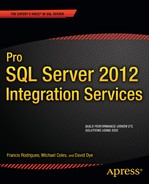
The Mapping page of the destination component, shown in Figure 14-5, shows you how the input columns match up with their destination column in SQL. This mapping pairs an input column, on the left, with a destination table column on the right. If there are data type or definition mismatches, you have the option of modifying the mapping to allow for different columns. This page is especially handy when dealing with Data Conversion transformations. Because the SSIS tries to automatically match based on the columns, the converted columns are usually not the ones mapped to the destination columns.
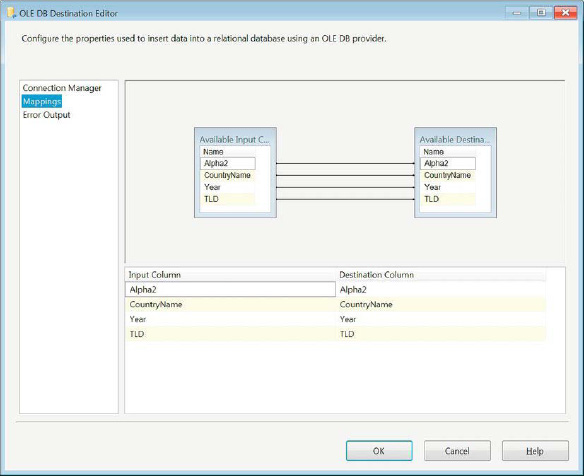
Figure 14-5. Mapping page of the OLE DB Destination Editor
In addition to the OLE DB destination, SSIS provides a SQL Server–specific bulk-load destination component, SQL Server Destination. This component bulk-loads the data into tables and views, but only if they exist on the same machine where the package is being executed. This is a huge limitation, and in the notes for the destination, Microsoft recommends using the OLE DB component instead. The editor for the component is very similar to the OLE DB destination, except it does not provide any options other than the connection manager, the table or view to load the data, and the mapping page.
Other RDBMS Sources and Destinations
For relational database management systems (RDBMSs) other than SQL Server, Microsoft provides drivers that are tuned for extracting data. For SSIS 11, the providers for these other systems have been developed by Attunity. (In prior versions, Attunity provided the drivers for Oracle connectivity.) The Source Assistant, shown in Figure 14-6, provides you with information on how to acquire providers for connectivity that do not come by default. For some of these providers, it is possible that the owner will charge you a fee for the use of their drivers.
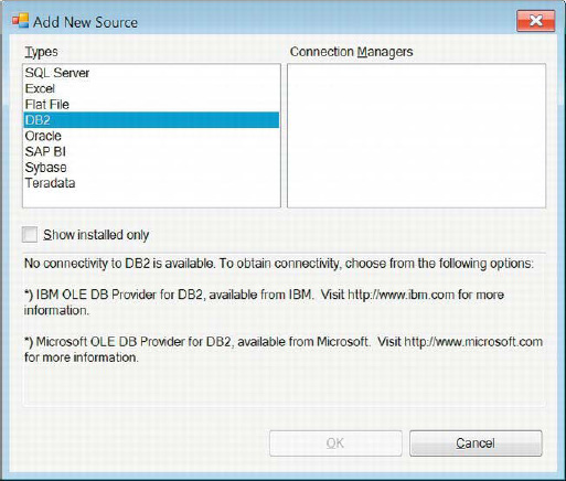
Figure 14-6. Providers for heterogenous sources
One of the pitfalls of using non–SQL Server connections is forgetting to ensure that the SQL variant is recognized by the provider. Some providers do not recognize the statement terminator (;), while others parse through the provided query as if it were a single line of code even though the text editor shows the new lines and formatting. In the second case, you will have to be conscious of how you comment out lines of code. You will have to use the multiline comment rather than a single-line comment.
When using different storage systems to source your data, we recommend using a Data Conversion transformation immediately after the source component. This will allow you to utilize the Union All transformation and other transformations without having to worry about data type mismatches between the datasets.
Flat File Sources and Destinations
Flat files are usually generated as an output process of a data dump. These flat files can be used as data storage, but they lack many of the advantages provided by RDBMSs. One of the appeals of keeping flat files around, however, is that security does not have to be necessarily as constricting as the database systems. They may offer quick access to the data without having an impact on the server that is hosting the data in a database system. The downsides to the flat files are that they cannot be queried, there are no means to maintain data integrity, and data quality maintenance measures do not exist. All of these advantages would have to be enforced on the database system from where the flat files are sourced, if such systems exist.
Using a flat file as a source requires the use of a Flat File Connection Manager. The connection manager is thoroughly discussed in Chapter 4. Using the properties defined in the connection manager, the source component acquires all the metadata required to extract the data. Figure 14-7 shows the options available with the Flat File Source Editor. The editor uses the configuration of the connection manager to collect the column information as well. As described in Chapter 4, the Flat File Connection Manager stores information such as the column and row delimiters, the column names, the column data type information, and some other information about the file and its data. The Preview button shows a sample of the rows that are read by using the configuration defined in the connection manager. The Retain Null Values from the Source as Null Values in the Data Flow option will preserve nulls in the pipeline. The Columns page acquires all of its information from the connection manager.
Figure 14-7. Flat File Source Editor
Flat file destinations, on the other hand, can operate in the opposite direction. If the flat file itself does not exist, you will have to add a new Flat File Connection Manager to configure the output file. Figure 14-8 shows the Flat File Destination Editor and how it modifies the connection manager. The New button will create a new Flat File Connection Manager. This will automatically open a dialog box, Flat File Format, which is shown in Figure 14-9. Using the option chosen in this dialog box, the connection manager is automatically configured for the most part because of the knowledge it gains from being at the end of the data flow pipeline. The Update button, however, forces you to modify the connection manager directly rather than importing the configuration through the metadata. The mappings simply map the columns in the pipeline to the columns defined in the connection manager.
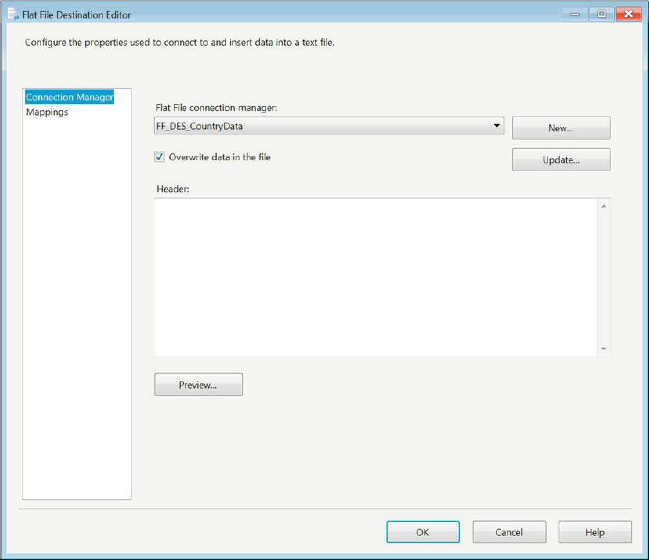
Figure 14-8. Flat File Destination Editor
The Flat File Format options allow you to define the layout of the flat file. Each of the options is covered in Chapter 4 for the Flat File Connection Manager section. The information for all nondelimited options is provided by the metadata stored in the pipeline.

Figure 14-9. Flat File Format dialog box
Excel Sources and Destinations
The appeal of Microsoft Excel stems from its worksheets’ similarity to database tables. Business users appreciate Excel for its ability to quickly display and modify tabular information. In the back end, Excel utilizes the Jet engine, the same engine behind Microsoft Access. This allows SSIS to execute certain SQL-like commands on the spreadsheet. The SQL interpretation of the Jet engine is nowhere as advanced as SQL Server’s, but it does have some rudimentary elements that can be used for ETL processes.
![]() NOTE: The Jet engine does not currently have a 64-bit provider. This may cause some issues as you try to manipulate spreadsheets using SSIS.
NOTE: The Jet engine does not currently have a 64-bit provider. This may cause some issues as you try to manipulate spreadsheets using SSIS.
The Excel source components are similar to the flat file source components, except for the dependency on the connection manager. The connection manager for the Excel file simply defines the folder path to its location. Figure 14-10 shows the Excel source component’s editor. The Connection Manager page allows you to choose the connection manager that points to the Excel file and one particular worksheet within that spreadsheet, or to provide a SQL query that will join different worksheets to return the desired data. The Jet engine does not allow the same leniency that other RDBMSs allow in terms of the data type matches on joins or null handling in data.

Figure 14-10. Excel Source Editor—SQL command textbox
Listing 14-2 provides the query that is used to extract the desired columns from a particular sheet. This query has the same advantages as using the SQL Command option in the OLE DB source component, in that the buffer is limited to only these four columns at the onset of the data flow. Figure 14-11 displays the Columns page, which allows you to choose the columns you wish to pass into the data flow. The difference between these two methods is that the by using the Table or View option, you are pulling all the available columns and then trimming them after SSIS has already processed the unwanted columns.
Listing 14-2. Excel Source SQL Command
SELECT Abbreviation,

   Capital,

   Flag,

   Lat

FROM   [Sheet1$]

Figure 14-11. Columns page of the Excel Source Editor
One of the difficulties with loading data into an Excel spreadsheet is eliminating prior rows that already exist within the worksheet (table/view). SSIS loads the spreadsheets incrementally by default. In order to reload the spreadsheet, you have to use an Execute SQL task within the control flow and point it to the destination Excel Connection Manager. Figure 14-12 shows the configuration of an Execute SQL task that can achieve this end.
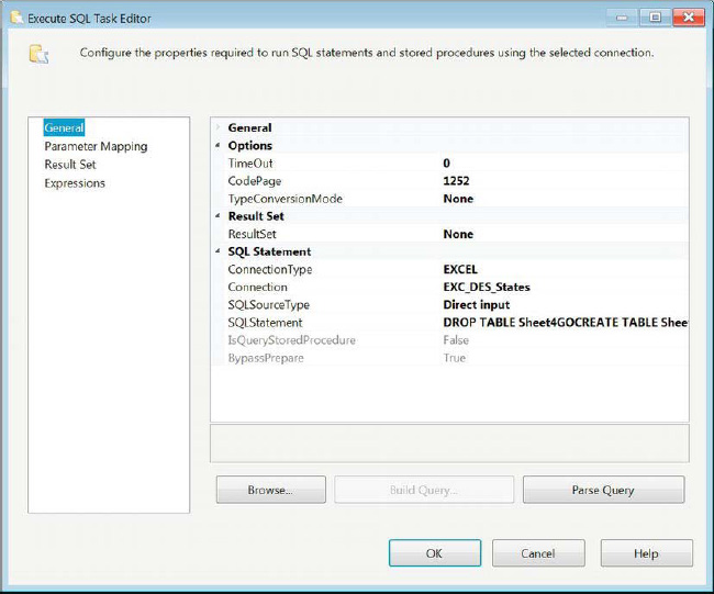
Figure 14-12. Execute SQL Task—truncate Excel worksheet
Listing 14-3 shows the actual SQL that is used to truncate an Excel worksheet. The original three spreadsheets will appear with a dollar sign ($) at the end of their names. In order to map the columns to the destination worksheet, it must exist in the file. The New button on the Excel destination component will generate the create script, just as the OLE DB destination generates a create table script. The Jet engine is extremely sensitive to keywords and will escape all the objects by placing single quotes around their names in the create script. This is similar to the OLE DB destination component escaping the objects by using square brackets around all the names.
Listing 14-3. Excel Worksheet Truncate Script
DROP TABLE Sheet4

GO


CREATE TABLE Sheet4(

    Abbreviation LongText,
Capital LongText,
Flag LongText,
Lat Double
)
GO
XML Sources
A great repository for metadata is an Extensible Markup Language (XML) file. XML files can be used to describe just about anything. XML serves many purposes: SQL Server’s XML functionality can output table records as XML; SSIS packages are essentially XML files that the dtexec.exe and Business Intelligence Development Studio interpret at runtime and design time, respectively; SQL Server stores extended properties of the objects in an XML, and other formats, including information not just related to ETL.
Figure 14-13 shows you the XML source editor that parses through an XML file by using an XML Schema Definition (XSD) to return the elements stored within the file. The Use inline schema will attempt to generate the XSD based on the values in the XML. However, if the XSD does not exist within the XML, the Generate XSD button will generate an XSD file for you. After the XSD is generated, it is created as its own file in the specified path. For this example, we used the upgrade log file of converting an SSIS 2008 project file to SSIS 2011 and generated an XSD for it.
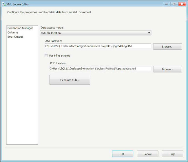
Figure 14-13. Connection Manager page of the XML Source Editor
Figure 14-14 shows the Columns page of the XML Source Editor. The interesting thing about this source component is that depending on the number of node levels of the XML, each gets its own output. The figure shows that this particular XML file has three levels: Property, Properties, and Event. The list is alphabetical and not hierarchical, so you cannot easily determine the structure just by looking at the outputs. Each output will have its column set based on the XSD.
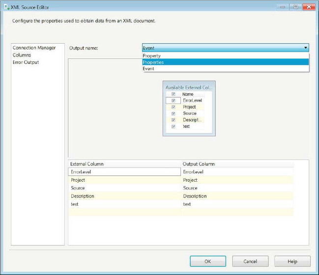
Figure 14-14. Columns page of the XML Source Editor
![]() NOTE: Along with an output for each of the node levels defined in the XSD, each of these outputs comes with its own error output that can be redirected as well.
NOTE: Along with an output for each of the node levels defined in the XSD, each of these outputs comes with its own error output that can be redirected as well.
Raw File Sources and Destinations
The raw file source and destinations provide an efficient method of storing data that doesn’t need to keep returning to the server at every request, such as Lookup transformations using the same dataset. These files should ideally be created on the local machine that is executing the package. One of the greatest advantages that these files provide is that if a query is used to return the same dataset multiple times, the query can be executed once and the result set stored in a file. At runtime, instead of each of the Lookup transformations querying the database, the result can be acquired directly off the machine.
Figure 14-15 shows the editor of the raw file destination. This component works in a slightly different way from the other sources and destinations in that the file needs to be loaded before it can provide any metadata as a source. It also does not utilize a connection manager in order to connect to a file.
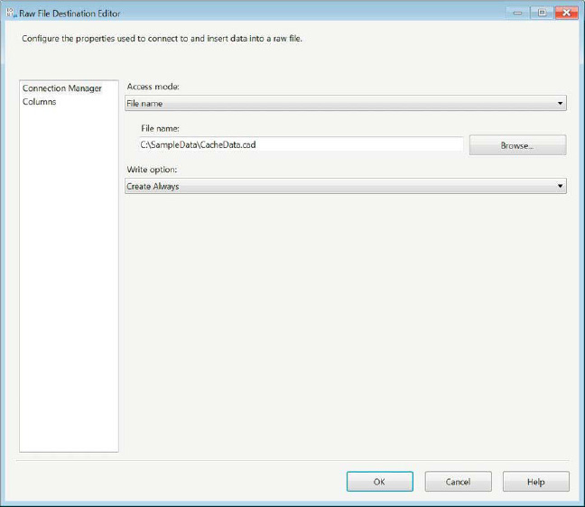
Figure 14-15. Raw File Destination Editor
After the data is loaded into the file, you can freely access it as a part of your process. Figure 14-16 shows the source component for the raw file. Just like the destination component, this component does not rely on a connection manager to identify the file it needs to reference. It can read the data right off the local machine and load into other destinations.

Figure 14-16. Raw File Source Editor
SQL Server Analysis Services Sources
Analysis Services cubes are analytical structures often used in the business intelligence field. Their greatest asset is the ability to store large numbers of aggregations so that querying might be faster. The cube itself can be queried only by using Multidimensional Expressions (MDX). The data types returned by these expressions do not always translate easily into database data types, so it is often the case that SSIS will simply cast them as character fields. There is an SSAS OLE DB provider that allows you to connect to a cube and extract certain values from the defined connection. Figure 14-17 shows the OLE DB source component that was used to query a cube.

Figure 14-17. SSAS OLE DB Editorwith MDX
The expression in the source component, replicated as Listing 14-4, is a simple MDX query that shows the number of calls that were placed to each call center. This query does not use any filters (MDX WHERE clauses) or cross joins to slice by multiple items. This query objective is simple and can translate into a GROUP BY SQL statement with a COUNT (DISTINCT CallID) column.
Listing 14-4. MDX Sample from an SSAS Source Component
SELECT {[Measures].[Calls]} ON COLUMNS,

 {[Fact Call Center].[Fact Call Center ID].[Fact Call Center ID]} ON ROWS

FROM [Adventure Works DW Denali]
![]() CAUTION: Unlike an SQL query, SSIS can get metadata from an MDX query only if it returns a dataset. If you use a filter with no data or return an empty set, SSIS will throw a metadata validation error. This can happen at design time as well as at runtime.
CAUTION: Unlike an SQL query, SSIS can get metadata from an MDX query only if it returns a dataset. If you use a filter with no data or return an empty set, SSIS will throw a metadata validation error. This can happen at design time as well as at runtime.
Recordset Destination
SSIS variables can often be used to hold data. In most cases, this data takes the form of scalar values, but in some instances an ADO.NET in-memory recordset is required. The SSIS Object type variables can be used to store tabular datasets to enumerate through the loop containers and provide additional functionality in conjunction with script components, as well as quick debugging assistants. After the recordset is stored inside the variable, the script component can be used to access the data with either C# or VB.
Figure 14-18 shows the editor of the recordset destination. The only editor for this component is the Advanced Editor. The VariableName property selects which SSIS variable will store the incoming data. The Input Columns tab is important as well because you need to identify the columns you wish to include in the variable. SSIS will not select all the columns by default. It will give you a warning until you specify the columns you require. This may sound cumbersome at first, but when used properly, it will prevent the variables from being bloated by unnecessary data.

Figure 14-18. Advanced Editor for Recordset Destination
Summary
SQL Server Integration Services 11 offers the capabilities to access data that is stored in many forms. Using the different providers, you can extract your data from a wide range of RDBMSs or flat files. The providers also allow you to insert the data in just about any storage form. This chapter introduced you to the methods of storage that SSIS can extract from and load. The next chapter dives into optimizing and tuning your data flows.