
C H A P T E R 8
Data Flow Transformations
The goal is to transform data into information, and information into insight.
—Carly Fiorina
In the previous chapter, you looked at how SSIS pulls data from point A and pushes it out to point B. In this chapter, you’ll begin exploring the different types of data manipulations, referred to as transformations, which you can perform on your data as it moves from its source to its destination. As Carly Fiorina indicated, our ultimate goal is to start with raw data and use it to reach a state of insight. Data flow transformations are the key to moving your raw data along the first half of that journey, turning it into usable information.
High-Level Data Flow
The SSIS data flow consists of sources, transformations, and destinations. Figure 8-1 shows the high-level view of SSIS’s data flow.
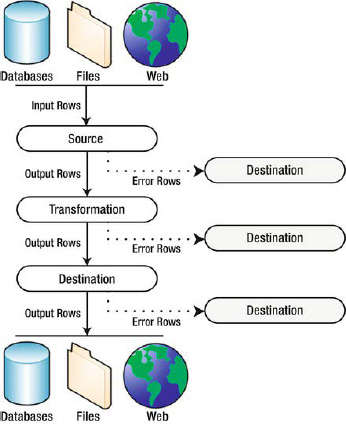
Figure 8-1. High-level overview of the SSIS data flow
As you can see from the diagram, SSIS source components pull data from a variety of sources such as databases, files, and the Web. The source component introduces data into the data flow, where it moves from transformation to transformation. After the data has been processed, it moves on to the destination component, which pushes it out to storage, including databases, files, the Web, or any other type of destination you can access. The solid black arrows in the diagram are analogous to the output paths (green arrows) in the SSIS designer. Some components, such as the Multicast transformation we discuss later in this chapter, have more than one output path.
Each type of data flow component (source components, transformations, and destination components) can also have an error output path. These are represented by red arrows in the BIDS designer. When a component runs into a data error while processing a row of data, the erroneous row is redirected to the error output. Generally, you’ll want to connect the error output to a destination component to save error rows for later review, modification, and possible reprocessing.
Types of Transformations
SSIS comes with 30 stock transformations out of the box. These standard transformations give you the power to manipulate your data in any number of ways, including modifying, joining, routing, and performing calculations on individual rows or entire rowsets.
Transformations can be grouped along functional lines, which we’ve done in this chapter. Row transformations and Split and Join transformations are two of the groups we cover, for instance. On a different level, transformations are also classified by how they process data. In particular, data flow transformations can be classified as either synchronous or asynchronous. In addition, they can be further subdivided by their blocking behavior.
Synchronous Transformations
Synchronous transformations process each row of input at the time. When sending data through a synchronous transformation, SSIS uses the input buffer (an area of memory set aside for temporary data storage during processing) as the output buffer. This is shown in Figure 8-2.

Figure 8-2. Synchronous transformations use the input buffer as the output buffer.
Because synchronous transformations reuse the input buffers as the output buffers, they tend to use less memory than asynchronous transformations. Generally speaking, synchronous transformations also share these other properties (though these don’t always hold true for every component):
- Synchronous components generally are nonblocking or only partially blocking. This means they tend to process rows and output them immediately after processing, or they process and output rows with minimal delay.
- Synchronous components also tend to output the same number of rows that they receive as input. However, some synchronous components may effectively discard rows, resulting in fewer output rows than input rows.
Asynchronous Transformations
Asynchronous transformations tend to transform data in sets. Asynchronous transformations are used when your method for processing a single row of data is dependent on other rows of data in your input. You may need to sort or aggregate your input data, for instance. In these situations, the transformation needs to see all rows of data at once, and can’t transform each row independently.
From a technical perspective, asynchronous transformations maintain separate input and output buffers. Data moves into the input buffers, is transformed, and then moved to the output buffers. The extra data movement between input and output buffers can cost you some performance, and the maintenance of two separate sets of buffers tends to use more memory than synchronous transformations. Figure 8-3 shows data moving between input and output buffers of an asynchronous transformation.

Figure 8-3. Asynchronous transformations move data from an input buffer to a separate output buffer.
In general, asynchronous transformations are designed to handle situations such as the following:
- The number of input rows does not equal the number of output rows. This is the case with the Aggregate and Row Sampling transformations.
- Multiple input and output buffers have to be acquired to queue up data for processing, as with the Sort transformation.
- Multiple rows of input have to be combined, such as with the Union All and Merge transformations.
Blocking Transformations
In addition to grouping transformations in synchronous and asynchronous categories, they can also be further subdivided by their blocking behavior, as noted earlier. Transformations that are fully blocking have to queue up and process entire rowsets before they can allow data to flow through. Consider the Sort transformation, which sorts an entire rowset. Consider pushing 1,000 rows through the Sort transformation. It can’t sort just the first 100 rows and start sending rows to output—the Sort transformation must queue up all 1,000 rows in order to sort them. Because it stops data from flowing through the pipeline while it is queuing input, the Sort transformation is fully blocking.
Some transformations hold up the pipeline flow for shorter periods of time while they queue up and process data. These transformations are classified as partially blocking. The Merge Join transformation is an example of a partially blocking transformation. The Merge Join accepts two sorted rowsets as inputs; performs a full, left, or inner join of the two inputs; and then outputs the joined rowsets. As data passes through the Merge Join, previously buffered rows can be discarded from the input buffers. Because it has to queue up a limited number of rows from each rowset to perform the join, the Merge Join is a partially blocking component.
Nonblocking transformations don’t hold up data flows. They transform and output rows as quickly as they are received. The Derived Column transformation is an example of a nonblocking transformation. Table 8-1 compares the properties of each class of blocking transformations.

Row Transformations
Row transformations are generally the simplest and fastest type of transformation. They are synchronous (with the possible exception of some Script Component transformations) and operate on individual rows of data. This section presents the stock row transformations available in SSIS.
![]() NOTE: We discuss the script component in detail in Chapter 10.
NOTE: We discuss the script component in detail in Chapter 10.
Data Conversion
A common task in ETL is converting data from one type to another. As an example, you may read in Unicode strings that you need to convert to a non-Unicode encoding, or you may need to convert numeric data to strings, and vice versa. This is what the Data Conversion transformation was designed for.
The Data Conversion transformation provides a simple way to convert the data type of your input columns. For our sample, we borrowed some data from the New York City Health Department. We took the data for selected restaurants that had dozens of health violations and saved it in an Excel spreadsheet. As you can see in Figure 8-4, we added a Data Conversion transformation immediately after the Excel source adapter.
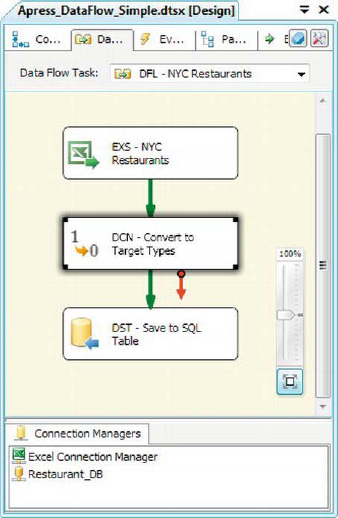
Figure 8-4. Using the Data Conversion transformation on an Excel spreadsheet
We’re using the Data Conversion transformation in the data flow because the Excel Connection Manager understands only a handful of data types. For instance, it can read character data only as Unicode data with a length of either 255 characters or as a 2.1 GB character large object (LOB). In addition, numbers are recognized only as double-precision floating-point numbers, so you have to explicitly convert them to other data types.
The Data Conversion transformation creates copies of columns that you indicate for conversion to a new data type. The default name for each newly created column takes the form Copy of <column name>, but as you can see in Figure 8-5, you can rename the columns in the Output Alias field of the editor. The Data Type field of the editor lets you choose the target data type for the conversion. In this case, we chose to convert the Violation Points column to a signed integer (DT_I4) and Unicode string columns to non-Unicode strings of varying lengths.

Figure 8-5. Editing the Data Converstion transformation
For purposes of data conversion especially, it’s important to understand how SSIS data types map to your destination data types. Microsoft Books Online (BOL) documents mappings between SSIS data types and a handful of RDBMSs. We provide an abbreviated list of mappings of SSIS to SQL Server data types and additional conversion options in Table 8-2.
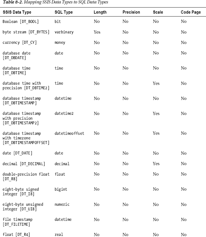

Note that SSIS data types can be mapped to additional data types not indicated here, such as the byte stream [DT_BYTES] data type, which can be mapped to varbinary, binary, uniqueidentifier, geography, and geometry data types. Some of the SSIS data types, such as the SSIS-provided unsigned integers, are not natively supported by SQL Server, but we’ve provided approximations in this table for data types that can be used to store other data types in SQL Server.
![]() TIP: The Derived Column transformation can perform the same task as the Data Conversion transformation, and more. In fact, you can think of Data Conversion as a convenience transformation that provides a subset of Derived Column functionality. Derived Column is far more flexible than Data Conversion but is a little more complex because you have to write your data type conversion using SSIS Expression Language cast operators. We discuss the Derived Column transformation later in this chapter and dig into the details of the SSIS Expression Language in Chapter 9.
TIP: The Derived Column transformation can perform the same task as the Data Conversion transformation, and more. In fact, you can think of Data Conversion as a convenience transformation that provides a subset of Derived Column functionality. Derived Column is far more flexible than Data Conversion but is a little more complex because you have to write your data type conversion using SSIS Expression Language cast operators. We discuss the Derived Column transformation later in this chapter and dig into the details of the SSIS Expression Language in Chapter 9.
Character Map
The Character Map transformation allows you to perform character operations on string columns. This example expands the previous one by adding a character map to change the case of the string columns, as shown in Figure 8-6.
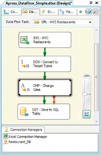
Figure 8-6. Character Map transformation in the data flow
![]() NOTE: Like the Data Conversion transformation, some of the functionality (uppercase and lowercase options) in the Character Map transformation can be performed by using Derived Column instead. We’ll look at Derived Column later in this chapter.
NOTE: Like the Data Conversion transformation, some of the functionality (uppercase and lowercase options) in the Character Map transformation can be performed by using Derived Column instead. We’ll look at Derived Column later in this chapter.
The Character Map transformation lets you apply string operations to inbound character data columns. For each selected column, you can choose one or more string operations to perform, such as converting a string to uppercase or lowercase. The Character Map Transformation Editor is relatively simple.
In this editor, you select the columns you wish to update. You then decide whether the result of the operation should be placed in a new column or just replace the value in the same column (in-place change). You can change the name of the output column by changing the value in the Output Alias field. Finally, in the Operation field, you can choose the types of transformations to apply to the selected columns. Figure 8-7 shows the transformation editor.
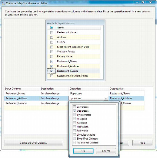
Figure 8-7. Editing the Character Map transformation
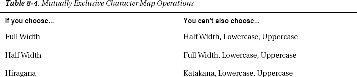
The Character Map transformation supports 10 string transformations you can perform on inbound data. You can choose more than one from the drop-down list to perform multiple transformations on an input column at once. In this example, we chose to use Uppercase selected string columns. The string operations you can choose from this transformation are listed in Table 8-3.

Although you can choose more than one operation on a single column, some of these transformations are mutually exclusive, as shown in Table 8-4.
Copy Column
The Copy Column transformation creates copies of columns you designate. Figure 8-8 extends the example we’ve been working on to include a Copy Column transformation.

Figure 8-8. Adding Copy Column to the data flow
The editor for this transformation is simple: just check off the columns you want to copy. The duplicated columns are named Copy of <column name> by default. You can edit the Output Alias field to change this to a more meaningful name if you choose to. The Copy Column transformation we’ve added will create a copy of the Picture Name column, as you can see in Figure 8-9.

Figure 8-9. Editing the Copy Column transformation in the editor
Derived Column
The Derived Column transformation is one of the most widely used, and flexible, row transformations available in SSIS. This transformation lets you create new columns, or replace existing columns, with values calculated from expressions that you create with the SSIS Expression Language. The SSIS Expression Language sports a powerful and flexible syntax supporting mathematical operators and functions, data type conversions, conditional expressions, string manipulation, and null handling.
![]() NOTE: We dive into the details of the SSIS Expression Language in Chapter 9.
NOTE: We dive into the details of the SSIS Expression Language in Chapter 9.
To create a Derived Column transformation, we drag it from the toolbar and place it in the data flow between the source and destination. We’ll build on the previous example by adding a Derived Column transformation, as shown in Figure 8-10.

Figure 8-10. Derived Column transformation in a simple data flow
The Derived Column transformation lets us define expressions, the results of which will be added to the output in new columns (or will replace existing columns). Figure 8-11 shows the Derived Column Transformation Editor as it appears in this example.

Figure 8-11. Editing the Derived Column transformation
As you can see in the transformation editor, two columns have their values replaced with the results of expressions. The new columns are populated with the results of expressions, which are written in the SSIS Expression Language. This powerful language lets you perform mathematical calculations and string manipulation on variables, columns, and constants. The expressions we used for the Picture Name and Copy of Picture Name columns look like this:
Picture Name  "C:\SampleData\" + [Picture Name]


Backup Picture Name  "C:\SampleData\Backup\" + [Picture Name]
These expressions use the string concatenation feature of SSIS Expression Language to prepend a file path to the picture name passed into the transformation. SSIS Expression Language uses C#-style syntax, including escape characters, which is why we had to double up the backslashes () in the expressions. The result is two full paths to files in the file system. Although these expressions are fairly simple and straightforward, we implemented a more complex derived column that calculates a letter grade based on the NYC Health Department grading scale. The result is stored in a new column that is added to the data flow, called Grade:
Grade (Restaurant_Violation_Points >= 28)?"C":(Restaurant_Violation_Points >= 14)?"B":"A"
This expression uses the conditional operator (?:) to assign a grade to each restaurant based on the NYC Health Department grading scale. This scale assigns a grade of A to restaurants with 0 to 13 violation points, B to restaurants with 14 to 27 violation points, and C to restaurants with 28+ points. The conditional operators in this example model those rules exactly.
As you read the expression from left to right, you’ll notice the first Boolean expression (Restaurant_Violation_Points >= 28), which returns True or False. If the result is true, the conditional operator returns the value after the question mark (C, in this case). If the result is false, the second Boolean expression, (Restaurant_Violation_Points >= 14), is evaluated. If it returns True, B is returned; if False, A is returned.
![]() NOTE: The SSIS Expression Language is a powerful feature of SSIS. If you’re not familiar with the functions and operators we’ve used in this example, don’t fret. We cover these and more in a detailed discussion of the SSIS Expression Language in Chapter 9.
NOTE: The SSIS Expression Language is a powerful feature of SSIS. If you’re not familiar with the functions and operators we’ve used in this example, don’t fret. We cover these and more in a detailed discussion of the SSIS Expression Language in Chapter 9.
Import Column
The Import Column transformation provides a way to enrich your rows in the data flow with LOB data from the file system. Import Column allows you to add image, binary, and text files to your data. We added an Import Column transformation to the data flow in Figure 8-12 to import images of restaurants on this list.
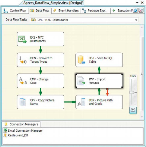
Figure 8-12. Import Column transformation in the data flow
The Import Column transformation is useful when you need to tie LOB data to rows of other data and store both in the database together. One caveat though—this transformation has one of the more arcane editors of any transformation. The first step to configuring Import Column is to select a string column on the Input Columns tab. We selected the Picture Name column that we previously populated with a full path to each image coming through the data flow (in the Derived Column transformation). You can see this in Figure 8-13.
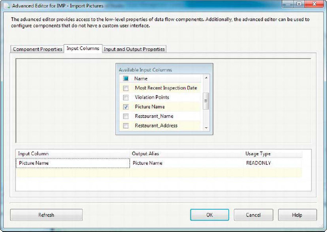
Figure 8-13. Choosing the input column that points to the file to be imported
The input column you choose in the first step tells the Import Column transformation which file to import into the data flow. As in our example, the task should contain a full path to the file.
The next step to configure this transformation is to add an output column to the Input and Output Properties. This column will hold the contents of the file after the Import Column reads it in. The following are appropriate data types for this new output column:
image [DT_IMAGE]for binary data such as images, word processing files, or spreadsheetstext stream [DT_TEXT]for text data such as ASCII text filesUnicode text stream [DT_NTEXT]for Unicode text data such as Unicode text files and UTF-16 encoded XML files
One of the more arcane aspects of Import Column is the configuration of the input column on the Input and Output Properties tab. To configure the input column, grab a pen and paper (yes, a pen and paper!) and write down the number you see next to the ID property for your output column. In our example, the number is 201.
Then edit the input column on the same tab. Scroll to the bottom of the page and type the number you just wrote down into the FileDataColumnID property. If you’re loading Unicode data, you can set the ExpectBOM property to True if your data has a byte order mark (BOM), or False if it doesn’t. This is shown in Figure 8-14.
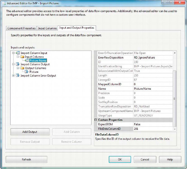
Figure 8-14. Finishing up configuration of the Import Column transformation
Finally, if you expect your input column to have nulls in it, you may want to change the ErrorRowDisposition property from the default RD_FailComponent to RD_IgnoreFailure or RD_RedirectRow. If RD_IgnoreFailure or RD_RedirectRow is set, the component will not throw an exception if it hits a null. Unfortunately, there’s no way for this component to handle nulls separately from actual file paths that don’t exist (you can handle this separately with additional data flow components if you want). The end result of properly configuring Import Column is that the data contained in the image files referenced by the input column are added to the data flow’s new output column.
HANDLING ERROR ROWS
OLE DB Command
The OLE DB Command transformation is an interesting row transformation that executes a SQL statement for each and every row that passes through the transformation. Most often, you’ll see the OLE DB Command transformation used to issue update statements against individual rows, primarily because SSIS doesn’t yet have a Merge Destination that will do the job for you in a bulk update.
![]() NOTE: The OLE DB Command transformation uses a processing model known as Row by Agonizing Row, or RBAR (a term popularized by SQL guru and Microsoft MVP Jeff Moden). In terms of SQL, this is not considered a best practice for large sets of data.
NOTE: The OLE DB Command transformation uses a processing model known as Row by Agonizing Row, or RBAR (a term popularized by SQL guru and Microsoft MVP Jeff Moden). In terms of SQL, this is not considered a best practice for large sets of data.
To demonstrate, we set up a data flow that reads an Excel spreadsheet containing updates to the restaurant information we loaded earlier and then applies the updates to the database. Figure 8-15 shows OLE DB Command in the data flow.

Figure 8-15. Data flow with an OLE DB Command transformation
All changes to the OLE DB Command transformation are made in an Advanced Editor window with four tabs. The Connection Managers tab lets you choose the OLE DB Connection Manager the transformation will issue SQL statements against. In Figure 8-16, the Restaurant_DB connection manager is selected.
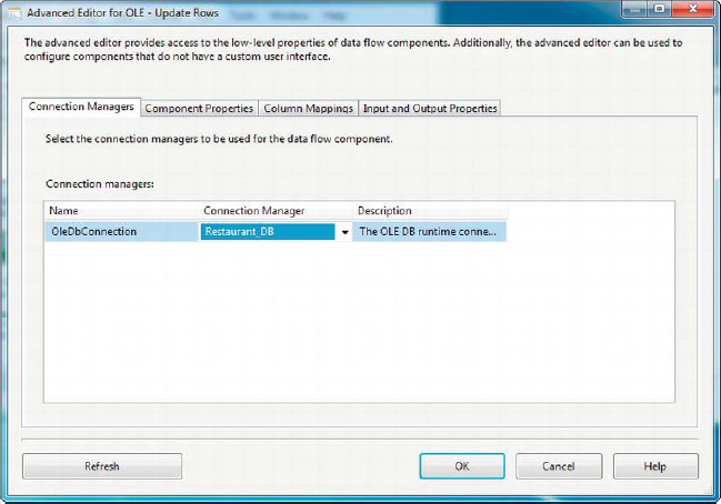
Figure 8-16. Connection Managers tab of the Advanced Editor for OLE
The Component Properties tab lets you set the SqlCommand property of the OLE DB Command transformation. The SqlCommand property holds the SQL statement you want executed against each row passing through the transformation. You can edit the SqlCommand property with the String Value Editor dialog box, accessed from the Component Properties tab, as shown in Figure 8-17. In this instance, we’ve set it to a simple parameterized UPDATE statement.
PARAMETERIZED SQL STATEMENTS
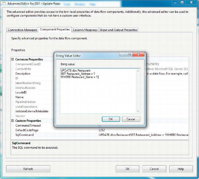
Figure 8-17. Component Properties tab of the Advanced Editor for OLE
The Column Mappings tab of the editor lets you map the OLE DB Command’s inbound columns to the parameters in your SQL statement. Because the OLE DB Command uses the question mark as a placeholder for parameters, the parameters are considered positional—that is, they can be referenced by their numeric position beginning at zero. Figure 8-18 shows that we mapped the Address String column to Param_0, and the Restaurant Name String column to Param_1.

Figure 8-18. Mapping inbound columns to OLE DB Command parameters in the Advanced Editor
The OLE DB Command is useful for some very specific situations you may encounter. However, the performance can be lacking, especially for large datasets (thousands of rows or more). We recommend using set-based solutions instead of the OLE DB Command transformation when possible, and minimizing the number of rows you send through OLE DB Command when you do have to use it.
Export Column
The Export Column transformation performs the opposite function of the Import Column transformation. Export Column allows you to extract LOB data from your data flow and save it to files in the file system. Figure 8-19 shows the Export Column transformation in the data flow.
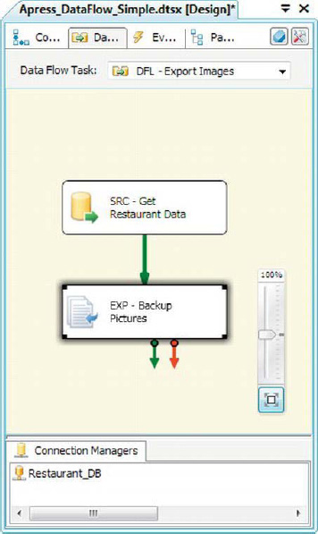
Figure 8-19. The Export Column transformation in the data flow
Though the Import Column and Export Column transformations are a matched pair, Export Column is much simpler to configure. The Export Column editor allows you to choose the column containing your LOB data with the Extract Column property and the destination file path in the File Path Column property. You can also choose from three check box properties: Allow Append will append your LOB data to the output file if the target file already exists, Force Truncate clears the target file before it starts writing data (if the file already exists), and Write Byte-Order Mark outputs a BOM to the output file, which can be important in situations when your LOB data consists of Unicode character data. Figure 8-20 shows the Export Column Transformation Editor.
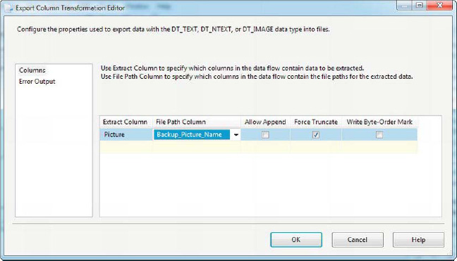
Figure 8-20. Configuring the Export Column transformation
Script Component
The script component lets you use your .NET programming skills to easily create SSIS components to fulfill requirements that are outside the bounds of the stock components. The script component excels at performing the types of transformations that other SSIS stock components do not perform.
With the script component, you can perform simple transformations such as counting rows in the data flow or extremely complex transformations such as calculating cryptographic one-way hashes and performing complex aggregations. The script component supports both synchronous and asynchronous modes, and it can be used as a source, destination, or in-flow transformation.
In this introduction, we’ll demonstrate a simple row counting, as illustrated in Figure 8-21.
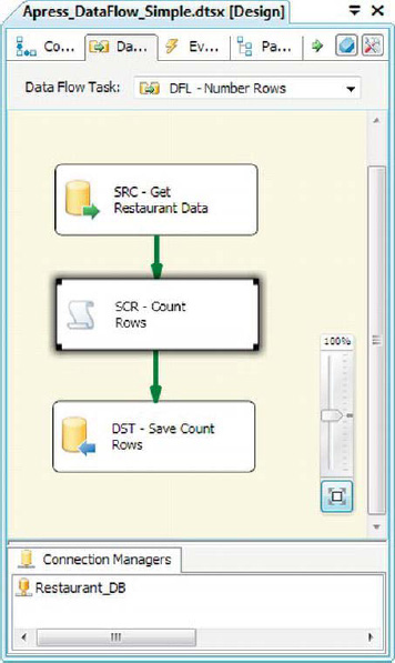
Figure 8-21. Script Component transformation in the data flow
In this example, we’ve used the script component to create a simple synchronous transformation that adds an increasing row number to each of the rows passed through it. To create this transformation, we dragged and dropped the script component from the SSIS Toolbox to the designer surface. It immediately prompted us for the type of component to create, as shown in Figure 8-22.

Figure 8-22. Choosing the type of script component to create
For this sample, we’re creating a simple synchronous transformation, so we chose the Transformation script component type. After the script component has been added to the data flow, we configured it through the Script Transformation Editor. We went to the Input Columns page first. On this page, you can choose the input columns, those columns that are accessible from within the script component. You can also indicate whether a column is read-only or read/write, as displayed in Figure 8-23.
![]() TIP: Chapter 10 covers how to create sources and destinations, as well as more-complex transformations, with the script component.
TIP: Chapter 10 covers how to create sources and destinations, as well as more-complex transformations, with the script component.

Figure 8-23. Choosing the input columns for the script component
Next we added a column to the component’s Output Columns collection on the Inputs and Outputs page of the editor. We called the column RowNumber and made it a four-byte signed integer [DT_I4], as shown in Figure 8-24.

Figure 8-24. Adding the RowNumber column to the script component’s output
As we mentioned, this component will be a simple synchronous script component. Script components are synchronous. by default. Whether or not a script component is synchronous is determined by the SynchronousInputID property on the output column collection of the Inputs and Outputs page. When this property is set to the name of an input column collection, as shown in Figure 8-25, the component is synchronous. If you set this property to None, the component is asynchronous. In this case, we set this property to the name of the input column collection, SCR - Count Rows.Inputs[Input 0].

Figure 8-25. Reviewing the SynchronousInputID property on the Inputs and Outputs page
Next we went to the Script page to edit the script. On this page, you can set the ScriptLanguage property to Microsoft Visual Basic 2008 or Microsoft Visual C# 2008. As you can see in Figure 8-26, we chose C# as our scripting language of choice. On the Script page, you can also choose any variables you want the script to access through the ReadOnlyVariables and ReadWriteVariables collections. We don’t use variables in this example, but we discuss them in detail in Chapter 9.

Figure 8-26. Editing properties on the Script page of the Script Transformation Editor
After we selected our scripting language, we edited the .NET script by clicking the Edit Scrip button. This pulls up the Visual Studio Tools for Applications (VSTA) Editor with a template for a basic synchronous script component, as shown in Figure 8-27.

Figure 8-27. Editing the script in the script component
All script components have a default class named ScriptMain, which inherits from the UserComponent class, which in turn inherits from the Microsoft.SqlServer.Dts.Pipeline.ScriptComponent class. The UserComponent class requires you to override three of its methods to implement a synchronous script component:
- The
PreExecute()method executes any setup code, such as variable initialization, before the component begins processing rows of data.PreExecute()is called exactly once when the component is first initialized. In this instance, we didn’t have any custom pre-execution code to run, so we just called thebase.PreExecute()method to perform any standard pre-execution code in the base class.- The
PostExecute()method executes any cleanup code, such as disposing of objects and assigning final values to SSIS variables, after the component has finished processing all rows of data.PostExecute()is called exactly once when the component has finished processing all data rows. Our sample didn’t require any custom post-execution code to run, so we called thebase.PostExecute()method to perform any standard post-execution code in the base class.- The
Input0_ProcessInputRow()method is the workhorse of the script component. This method is called once per input row. It accepts anInput0Bufferparameter with the contents of the current row in it. With thisInput0Bufferparameter, you can read and write values of input fields. In our example, we increment theRowNumbervariable with each call to the method and assign its value to theRowNumberfield of theInput0Buffer.
The result is a new column added to the data flow called RowNumber, which contains an incremental number for each row in the data flow. You can view the data in the data flow by adding a data viewer to the script component output. To do this, right-click the green arrow coming out of the script component and choose the Enable Data Viewer option from the context menu, as shown in Figure 8-28.

Figure 8-28. Enabling the data viewer on the script component output
After you’ve added the data viewer to the output path, you’ll see a magnifying glass icon appear on the output arrow, as shown in Figure 8-29.
Figure 8-29. Data viewer magnifying glass icon on output path
When you run the package, the data viewer will appear in a pop-up window with a grid containing data from the data flow. The data viewer holds up the data flow, so rows will not move on to the next step until you either click the arrow button or Detach. Clicking the arrow button allows another set of rows to pass through, after which it will pause the data flow again. The Detach button detaches the data viewer from the data flow, causing the data viewer to stop collecting and displaying new rows and allowing all rows to pass through. The results of placing the data viewer in our example package are shown in Figure 8-30.
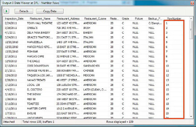
Figure 8-30. Looking at data in the data viewer
The data viewer is a very handy data-debugging tool, and one you’ll probably want to become familiar with—you’ll undoubtedly find yourself using it often to troubleshoot data flow issues and data errors.
![]() NOTE: Previous versions of SSIS included four types of data viewer—the Grid, Histogram, Scatterplot, and Column Chart data viewers. Because the Grid data viewer is the most commonly used, the SSIS team removed the other types of data viewers from SSIS 11.
NOTE: Previous versions of SSIS included four types of data viewer—the Grid, Histogram, Scatterplot, and Column Chart data viewers. Because the Grid data viewer is the most commonly used, the SSIS team removed the other types of data viewers from SSIS 11.
Rowset Transformations
Rowset transformations generate new rowsets from their input. The Rowset transformations are asynchronous, and the number of rows in the input is often not the same as the number of rows in the output. Also the “shape” of the output rowsets might not be the same as the shape of the input rowsets. The Pivot transformation—which we discuss later in this section—turns the input rowset on its side, for instance.
Aggregate
The Aggregate transformation performs two main tasks: (1) it can apply aggregate functions to your input data and (2) it allows you to group your data based on values in your input columns. Basically, it performs a function similar to the T-SQL aggregate functions (for example, MIN, MAX, COUNT) and the GROUP BY clause.
In the sample package shown in Figure 8-31, we are importing sample aviation incident data from the National Transportation Safety Board and perform two aggregations on the inbound data, each represented in the data flow by a different output from the Aggregate transformation.

Figure 8-31. Sample package with Aggregate transformation
The Aggregate transformation can be configured in Basic mode or Advanced mode. In Basic mode, the transformation has one output; in Advanced mode, it can have more than one output, each containing the result of a different aggregation. In this example, we have configured two aggregations:
- The first aggregation is called
AggByMonth. This aggregation sums the injury count fields in the input, and groups byEventYearandEventMonth.- The second aggregation is called
AggByState. This aggregation sums the injury count fields, grouping byState,EventYear, andEventMonth.
Figure 8-32 shows the Aggregate Transformation Editor.
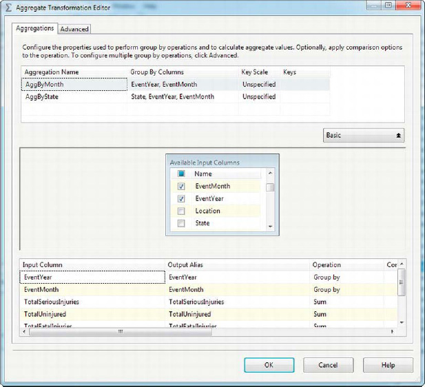
Figure 8-32. Editing the Aggregate transformation in Advanced mode
The Advanced/Basic button reveals or hides the multiple aggregation configuration box at the top of the editor. You can choose columns from the input column list and select the operations to perform on those columns in the lower portion of the editor. The operations you can choose include the following:
Group By groups results based on this column, just like the
GROUP BYclause in SQLSELECTqueries.Count returns the count of values in this column. Nlls are included in the count if you select
(*)as the input column. Otherwise, nulls are ignored. This operation is equivalent to the SQLCOUNTaggregate function.Count Distinct returns the count of distinct values in this column. Equivalent to the SQL
COUNT(DISTINCT ...)aggregate function.Sum returns the sum of the values in this column. Equivalent to the SQL
SUMaggregate function.Average returns the average of the values in the selected column. Equivalent to the SQL
AVGaggregate function.Minimum returns the minimum of values from the column. Equivalent to the SQL
MINaggregate function.Maximum returns the maximum of values from the column. Equivalent to the SQL
MAXaggregate function.
The Group By, Count, and Count Distinct operations can be performed on numeric or string data. The Sum, Average, Minimum, and Maximum operations can be performed on only numeric data.
![]() TIP: The Aggregate transformation does not require inbound data to be sorted.
TIP: The Aggregate transformation does not require inbound data to be sorted.
Sort
The Sort transformation sorts inbound rows based on the values from columns that you select in the designer. There are several reasons you may need to sort your input data in the data flow, including the following:
- Some transformations, such as Merge Join presented later in this chapter, require input data to be sorted.
- Under some circumstances, you can achieve better performance when saving data to a relational database when the data is presorted.
- In some instances, data needs to be processed in a specific order, or sorted before being handed off to another data flow or ETL process.
In any of these instances, you’ll need to sort your data prior to passing it on, as shown in Figure 8-33.
![]() TIP: Because Sort is a fully blocking asynchronous transformation, it will hold up the data flow until it has completed the sort operation. It’s a good idea to sort data at the source when possible. If you’re pulling data from a relational database, consider putting an
TIP: Because Sort is a fully blocking asynchronous transformation, it will hold up the data flow until it has completed the sort operation. It’s a good idea to sort data at the source when possible. If you’re pulling data from a relational database, consider putting an ORDER BY clause on your query to guarantee order, for instance. If the order of your input is not guaranteed—for instance, when you pull data from a flat file or perform transformations on your data that could change the order of your data in the data flow, the Sort transformation may be the best option. If your data is not indexed on the sort columns in SQL Server, an ORDER BY clause might use a lot of server-side resources. If, however, your data is indexed, the SSIS Sort transformation will not be able to take advantage of the index.
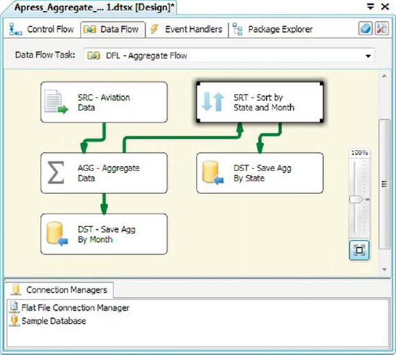
Figure 8-33. Sort transformation in data flow
The Sort transformation offers several options applicable to sorting. In the Sort editor, you can choose the columns that you want to sort by, and choose the Sort Type (ascending or descending options) and Sort Order for each column. The Sort Order indicates the order of the columns in the sort operation. In our example, we’re sorting by the State column, and then by EventYear and EventMonth.
The Comparison Flags option provides several sort-related options for character data, such as ignoring case and symbols during the sort process. In our example, we chose to ignore case on the State column when sorting the inbound data. You can also choose to remove rows with duplicate sort values. Figure 8-34 shows the Sort Transformation Editor.

Figure 8-34. Editing the Sort transformation
THE ISSORTED PROPERTY
One of the features of note in the Sort transformation is exposed in the Advanced Editor, via the Input and Output Properties. The IsSorted property is automatically set by the Sort transformation, as you can see in Figure 8-35.
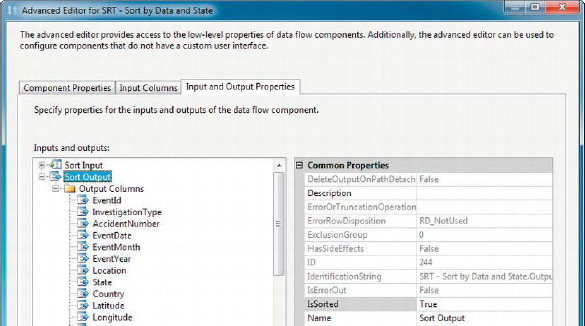
Figure 8-35. IsSorted property in Sort transformation Advanced Editor
This property is checked by transformations that require sorted input, such as Merge Join covered later in this chapter. If it’s not set to True on an output further up the data flow, the transformation requiring sorted input will complain about it.
Closely related to the IsSorted output property is the column-level SortKeyPosition property, which is shown in Figure 8-36.
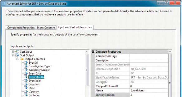
Figure 8-36. SortKeyPosition property in the Advanced Editor
For the Sort transformation, the SortKeyPosition can be set through the Basic Editor. If you presort your inbound data, as with an ORDER BY clause in a source query, you’ll have to set these properties on the source adapter manually.
Pivot
The Pivot transformation allows you to perform a pivot operation on your input data. A pivot operation means you take your data and “turn it sideways,” essentially turning values from a column into columns in the result set. As shown in Figure 8-37, we added a Pivot transformation to the data flow to denormalize our aggregated aviation data, creating columns with month names.
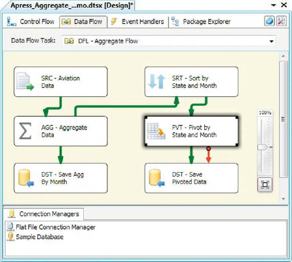
Figure 8-37. Adding a Pivot transformation to pivot aggregated aviation data
This Pivot transformation takes the individual rows of input and pivots them based on the EventMonth. The pivot operation turns the months into columns, as shown in Figure 8-38.

Figure 8-38. Result of Pivot transformation
In previous releases of SSIS, the Pivot Transformation Editor was difficult to work with—a situation that has been corrected in this new release. The newly redesigned Pivot Transformation Editor is shown in Figure 8-39.

Figure 8-39. Pivot Transformation Editor
![]() NOTE: The Pivot transformation requires input data to be sorted, or incorrect results may be produced. Unlike other transformations that require sorted input data, Pivot doesn’t enforce this requirement. Make sure your input to Pivot is sorted.
NOTE: The Pivot transformation requires input data to be sorted, or incorrect results may be produced. Unlike other transformations that require sorted input data, Pivot doesn’t enforce this requirement. Make sure your input to Pivot is sorted.
Percentage Sampling
The Percentage Sampling transformation selects a given percentage of sampled rows from the input to generate a sample dataset. This transformation actually splits your input data into two separate datasets—one representing the selected sampling of rows and another containing the rows from your dataset that were not selected for sampling. Figure 8-40 demonstrates a simple data flow that samples rows from the aviation flat file we’ve used in the examples in this section.
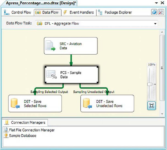
Figure 8-40. Percentage Sampling transformation in the data flow
As you can see in the data flow, the Percentage Sampling transformation splits your inbound dataset into two separate outputs:
Sampling Selected Output contains all the rows selected by the component for the sample set
Sampling Unselected Output contains the remaining rows that were not selected by the component for the sample set
The Percentage Sampling Transformation Editor makes it very easy to edit this transformation. Simply select the Percentage of Rows you wish to sample (the default is 10%), and change the names of the outputs if you want to. You can also set the random seed for the transformation. If you do not set the random seed, the component uses the operating system tick counter to randomly seed a selection of sample rows from your input data, so the sample dataset will change during each run. If you do set a random seed, the same sample dataset is generated each time (assuming the source data does not change between runs, of course). Figure 8-41 shows the Percentage Sampling Transformation Editor.
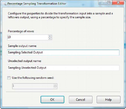
Figure 8-41. Editing the Percentage Sampling transformation
Percentage Sampling is useful when you want to train and test data-mining models, or if you want to efficiently test your ETL processes with a representative sample of input data.
![]() TIP: The Percentage Sampling Transformation Editor allows you to choose the percentage of rows to include in your sample, but keep in mind that because of the sampling algorithm used by SSIS, your sample dataset may be slightly larger or smaller than this percentage. This transformation is similar to the T-SQL
TIP: The Percentage Sampling Transformation Editor allows you to choose the percentage of rows to include in your sample, but keep in mind that because of the sampling algorithm used by SSIS, your sample dataset may be slightly larger or smaller than this percentage. This transformation is similar to the T-SQL TABLESAMPLE with PERCENT option.
Row Sampling
The Row Sampling transformation is similar to the Percentage Sampling transformation, except that you choose the number of rows to sample instead of the percentage of rows to sample. Figure 8-42 shows the Row Sampling transformation in the data flow.
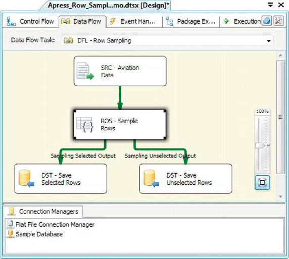
Figure 8-42. Row Sampling transformation in the data flow
The Row Sampling Transformation Editor, shown in Figure 8-43, is very similar to the Percentage Sampling editor. The only real difference is that with Row Sampling, you choose a number of rows instead of a percentage of rows to sample.

Figure 8-43. Row Sampling Transformation Editor
There is a slight behavior difference between the Percentage Sampling and Row Sampling transformations. With Percentage Sampling, you may end up with a sample set that is slightly larger or smaller than the percentage sample size you’ve requested. With Row Sampling, however, you’ll get exactly the number of rows you request, assuming you request a sample size that is less than the number of rows in the input dataset. If your sample size is equal to (or greater than) the number of rows in your input dataset, all rows are selected in the sample. The Row Sampling transformation is similar in functionality to the T-SQL TABLESAMPLE clause with ROWS option.
Unpivot
The Unpivot transformation normalizes denormalized datasets. This transformation takes selected columns from an input dataset and unpivots them into more-normalized rows. Taking the example of denormalized aviation data we used in the Pivot transformation example, we can Unpivot it back into a more normalized version, as shown in Figure 8-44.

Figure 8-44. Unpivoting a denormalized dataset
The Unpivot transformation is shown in the sample data flow in Figure 8-45.
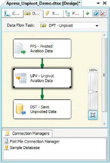
Figure 8-45. Unpivot transformation in sample data flow
Configuring the Unpivot transformation requires choosing the columns to unpivot and giving the newly unpivoted destination column and the pivot key value column names. Figure 8-46 shows the Unpivot Transformation Editor.

Figure 8-46. Unpivot Transformation Editor
In the editor, you select the columns you want to pivot from the Available Input Columns section. Any columns you don’t want to be pivoted are checked off as Pass Through columns. In the bottom-right corner, you choose a pivot key value column name—this is the name of the column you wish to place your pivot key values into. In this example, we chose the column name Month, and the pivot key values are the month names for each column.
If you choose to, you can change the pivot key values to something else, although they must all be unique. In our example, we went with the default, which is the same value as the Input Column name. We could, for instance, use the full month names (January, February, and so forth) as pivot key values.
The Destination Column is the name of the column you wish to place the unpivoted values into. In this case, the name is TotalMinorInjuries. The values for each unpivoted column are added in this newly created column.
![]() TIP: The Destination Column name must be the same for all your input columns.
TIP: The Destination Column name must be the same for all your input columns.
Splits and Joins
SSIS includes several transformations that allow you to split, merge, and join datasets in the data flow. These transformations are useful for combining multiple datasets, duplicating datasets, performing lookups, and creating copies of datasets.
Lookup
The Lookup transformation lets you enrich your data by retrieving related data from a reference dataset. Lookup is similar in functionality to a join operation in SQL Server. In the Lookup Transformation Editor, you choose the source data columns and the related columns from the reference dataset. You also choose the columns you wish to add to your data flow from the reference dataset. Figure 8-47 is a sample data flow that pulls in National Football League game data from a flat file and performs lookups against team data stored in a SQL Server database table.

Figure 8-47. Lookup transformations in a sample data flow
There are two lookups in this data flow: one looks up the winning team’s name, and the other looks up the losing team’s name. The LKP – Winner lookup was configured with the Lookup Transformation Editor, shown in Figure 8-48.
![]() TIP: If your reference data has multiple rows with the same values in the join key columns, duplicates are removed. SSIS will generate warning messages when duplicates are encountered. The reference data rows are considered in the order in which they are retrieved by the lookup component.
TIP: If your reference data has multiple rows with the same values in the join key columns, duplicates are removed. SSIS will generate warning messages when duplicates are encountered. The reference data rows are considered in the order in which they are retrieved by the lookup component.

Figure 8-48. General page of the Lookup Transformation Editor
The General page of the editor lets you choose the connection manager that will be the source of the reference data. Your options are an OLE DB Connection Manager or a Cache Connection Manager. For this sample, we went with the default OLE DB Connection Manager.
You can also choose the cache mode on this page. You have three options for cache mode:
Full Cache mode preloads and caches the entire reference dataset into memory. This is the most commonly used mode, and it works well for small reference datasets or datasets for which you expect a large number of reference rows to match.
Partial Cache mode doesn’t preload any reference data into memory. With this cache mode, reference data rows are retrieved from the database as they are needed and then cached for future lookups. Individual
SELECTstatements are issued to retrieve each data row. This mode is useful when you have a small reference dataset, or when you expect very few reference rows to match many records in the input dataset.No Cache mode doesn’t preload any reference data. In No Cache mode, reference data rows are retrieved as needed, one at a time using individual
SELECTstatements. Technically speaking, the No Cache mode does in fact cache the last reference row it retrieved, but discards it as soon as a new reference row is needed. This mode is normally not recommended unless you have a very small reference dataset and expect very few rows to match. The overhead incurred by this cache mode can hurt your performance.
The Lookup transformation is generally closely tied to the OLE DB Connection Manager. By default, the lookup wants to pull its reference data from an OLE DB source, such as a SQL Server or other relational database. When you want to pull reference data from another source, such as a flat file or Excel spreadsheet, you need to store it in a Cache transformation first. We cover the Cache transformation in the next section.
The final option on this first page lets you specify how to handle rows with no matching entries. You have four options:
Fail Component (default): If an input row passes through that does not have a matching row in the reference dataset, the component fails.
Ignore Failure: If an input row passes through that does not have a matching reference row, the component continues processing, setting the value of reference data output columns to null.
Redirect Rows to No Match Output: When this option is set, the transformation creates a “no match” output and directs any rows that don’t have matching reference rows to the new output.
Redirect Rows to Error Output: When this option is set, the component directs any rows with no matching reference rows to the transformation’s standard error output.
The Connection page of the editor lets you select an OLE DB Connection Manager that points to the database where your reference data is stored. On this tab, you also choose the source table or a SQL query, as shown in Figure 8-49.
![]() TIP: Specifying a SQL query instead of a table as your source is a best practice. There is less overhead involved when you specify a SQL query, because SSIS doesn’t have to retrieve table metadata. You can also minimize the amount of data retrieved with a SQL query (both columns and rows), and you can’t do that if you specify a table.
TIP: Specifying a SQL query instead of a table as your source is a best practice. There is less overhead involved when you specify a SQL query, because SSIS doesn’t have to retrieve table metadata. You can also minimize the amount of data retrieved with a SQL query (both columns and rows), and you can’t do that if you specify a table.
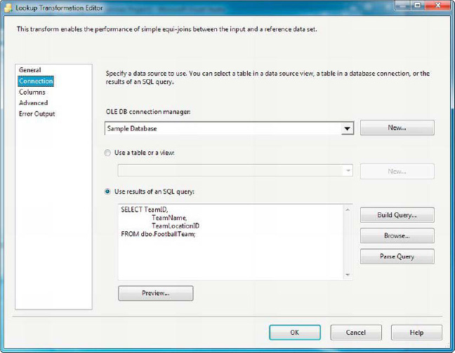
Figure 8-49. Connection page of the Lookup Transformation Editor
The third page of the editor—the Columns page—is where you define the join between your input dataset and your reference dataset. Simply click on a column in the Available Input Columns box and drag it to the corresponding column in the Available Lookup Columns box. Select the check boxes next to the reference data columns you wish to add to your data flow. Figure 8-50 shows the Columns page.
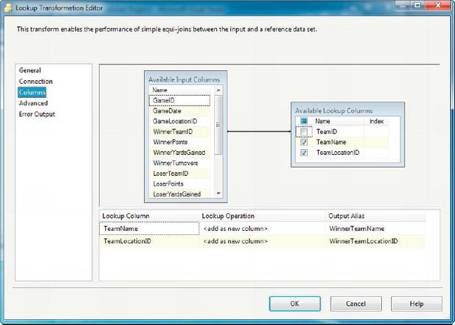
Figure 8-50. Columns page of the Lookup Transformation Editor
In this example, we joined the WinnerTeamID column of the input dataset to the TeamID column of the reference data, and chose to add TeamName and TeamLocationID to the destination. The columns you select from the Available Lookup Columns box are added to the grid in the lower portion of the editor. Each Lookup Column has a Lookup Operation assigned to it that can be set to <add as new column> or Replace ‘Column, indicating whether the column values should be added to the data flow as new columns or if they should replace existing columns. Finally, the Output Alias column allows you to change the name of the output column in the data flow.
The Advanced page lets you set Lookup caching properties. The Cache Size property indicates how much memory should be used for caching reference data. The maximum 32-bit cache size is 3,072 MB, and the maximum 64-bit cache size is 17,592,186,044,416 MB.
In Partial Cache mode, you can also set the Enable Cache for Rows with No Matching Entries option and set a percentage of allocation from the cache (default is 20%) on this tab. This option caches data values that don’t have matching reference rows, minimizing round-trip queries to the database server.
The Custom Query option lets you change the SQL query used to perform database lookups in Partial Cache or No Cache mode, as referenced in the figure below.
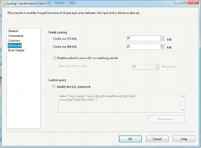
Figure 8-51. Advanced page of the Lookup Transformation Editor
Cache Transformation
As we mentioned in the previous section, the Lookup transformation, by default, looks for an OLE DB Connection Manager as its source for reference data. Other sources can be used, but they must be used indirectly via a Cache transformation. The Cache transformation can read data from a wide variety of sources, including flat files and ADO.NET data sources that aren’t supported directly by the Lookup transformation as illustrated in Figure 8-52.
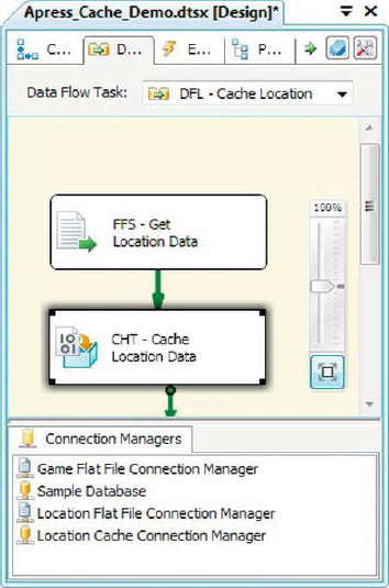
Figure 8-52. Populating the Cache transformation
As you can see in the figure, the Cache transformation accepts the output of a source component in the data flow as its input. It uses a Cache Connection Manager to cache the reference data in memory for use by the lookup component. Because the Cache transformation has to be populated before your lookup executes, you generally want to populate it in a separate data flow that precedes the data flow containing your lookups. In our sample, we populated the Cache transformation in one data flow, performed the lookup in a second data flow, and linked them with a precedence constraint, as shown in Figure 8-53.
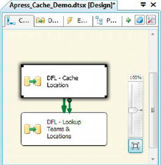
Figure 8-53. Populating the Cache transformation in a separate data flow
The Cache transformation is configured through the Cache Transformation Editor. The Connection Manager page lets you choose the Cache Connection Manager that will be populated with your cached reference data, as shown in Figure 8-54.

Figure 8-54. Connection Manager page of the Cache Transformation Editor
You can edit the Cache Connection Manager by clicking the Edit button to pull up the Connection Manager Editor. On the General tab of the editor, shown in Figure 8-55, you can change the name of the connection manager and choose to use a file cache. If you choose to use a file cache, the connection manager will write cached data to a file. You can also use an existing cache file as a source instead of pulling data from an upstream source in the data flow.

Figure 8-55. General tab of the Cache Connection Manager Editor
The Columns tab shows a list of the columns in the cache and their data types and related information. The Index Position column must be configured to reflect the columns you want to join in the lookup component. Columns that are not part of the index have an Index Position of 0; index columns should be numbered sequentially, beginning with 1. In our example, the LocationID column is the only index column, and is set to an Index Position of 1. Figure 8-56 shows the Columns tab.

Figure 8-56. Columns tab of the Cache Connection Manager Editor
Our sample package demonstrating the Cache transformation expands on the previous example by performing a lookup against the Cache transformation, as shown in Figure 8-57.
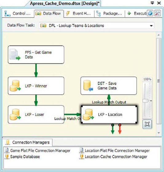
Figure 8-57. Data flow with Llokup against Cache transformation
The Lookup transformation against a cache is configured similarly to the lookup against an OLE DB source. The main differences are as follows:
- You must choose Full Cache mode. Partial Cache and No Cache are not valid options for lookups against a cache.
- The Connection type must be set to Cache Connection Manager.
- On the Connection tab of the Lookup transformation, you must choose a Cache Connection Manager instead of an OLE DB Connection Manager.
On the Columns tab, you’ll also notice a magnifying glass icon in the Index column of the Available Lookup Columns box, as shown in Figure 8-58. These columns are the columns you will map to your input data. Other than these minor differences, the operation of the lookup against a Cache Connection Manager is exactly the same as against an OLE DB source.

Figure 8-58. Columns tab of the Lookup transformation against a Cache Connection Manager
Conditional Split
The Conditional Split transformation lets you redirect rows of data that meet specific conditions to different outputs. You can use this functionality as a tool to direct data down different processing paths, much like an if...then...else construct in procedural programming languages (such as C# or VB), or as a filter to eliminate data from your dataset, as with the SQL WHERE clause. We’ve expanded the previous example to filter out any games that did not occur during the regular season, as shown in Figure 8-59.

Figure 8-59. Adding a Conditional Split transformation to the data flow
The Conditional Split Transformation Editor gives you control to add as many outputs as you like to the transformation. Each output has rows redirected to it based on the condition you provide for it. The condition is written in the form of an SSIS Expression Language expression. Often you’ll use variables or columns in your conditions, to make your data self-directing. In this example, we’ve added one output to the transformation called Regular Season Games. The condition we applied to this output is [GameWeek] == “Regular Season”, refer to Figure 8-60 below. We discuss the SSIS Expression Language in Chapter 9.

Figure 8-60. Editing the Conditional Split transformation
When the GameWeek column contains the value Regular Season, data is redirected to the Regular Season Games output. Note that string comparisons in SSIS Expression Language are case-sensitive. Any rows that do not match this condition are directed to the default output, which we’ve named Post Season Games in this example.
![]() TIP: When you define multiple outputs with conditions, they are evaluated in the order indicated by the Order field. As soon as a row matches a given condition, it is immediately redirected to the appropriate output, and no comparisons are made against subsequent conditions.
TIP: When you define multiple outputs with conditions, they are evaluated in the order indicated by the Order field. As soon as a row matches a given condition, it is immediately redirected to the appropriate output, and no comparisons are made against subsequent conditions.
When you connect the output of the Conditional Split transformation to the input of another data flow component, you’ll be presented with an Input Output Selection box. Choose which output you want to send to the next component, as shown in Figure 8-61.
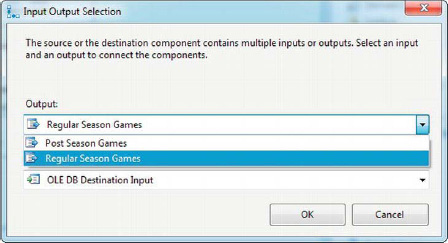
Figure 8-61. Input Output Selection when connecting the Conditional Split transformation
We didn’t connect the Post Season Games output to any downstream components in this case, which means the rows directed to it won’t be sent down the data flow. This is effectively a filter on the input data.
Multicast
The Multicast transformation duplicates your data in the data flow, which comes in very handy in many situations where you want to apply different transformations to the same source data in parallel, or when you want to send your data to multiple destinations simultaneously. To build on the previous sample, we’ve added a Multicast transformation just before the OLE DB destination in our data flow. We’ll use the Multicast transformation to send the transformed data to two destinations: the OLE DB destination and a flat file destination, as shown in Figure 8-62.

Figure 8-62. Multicast transformation sending data to multiple destinations
You can use the Multicast transformation to duplicate your data as many times as necessary, although it’s most often used to create one copy of its input data.
Union All
The Union All transformation combines the rows of two or more datasets into a single dataset, like the UNION ALL operator in SQL. For this sample, we’ve taken two flat files with daily weather data in them and combined them into a single dataset in the data flow, as shown in Figure 8-63.

Figure 8-63. Combining data from two source files with the Union All transformation
When you add the first input to the Union All transformation, it defines the structure of the output dataset. When you connect the second and subsequent inputs to the Union All transformation, they are lined up, column by column, based on matching column names. You can view the columns from all the inputs by double-clicking the Union All transformation to reveal the editor, as shown in Figure 8-64.

Figure 8-64. Union All Transformation Editor
The Output Column Name entries list the names of each column added to the output. The names are editable, so you can change them to your liking. If you have different names for columns that should be matched in the outputs, you can choose them from drop-down lists in the Union All Input lists. Choosing <ignore> will put a null in the column for that input.
![]() TIP: The output from the Union All transformation is not guaranteed to be in order when more than one input is involved. To guarantee order, you’ll need to perform a Sort after the Union All.
TIP: The output from the Union All transformation is not guaranteed to be in order when more than one input is involved. To guarantee order, you’ll need to perform a Sort after the Union All.
Merge
The Merge transformation is similar to the Union All, except that it guarantees ordered output. To provide this guarantee, the Merge transformation requires all inputs to be sorted. This is particularly useful when you have to merge inputs from two separate sources and then perform a Merge Join with the resulting dataset. Figure 8-65 shows the Merge transformation with two sorted inputs.

Figure 8-65. Merge transformation with two sorted inputs
In our example, we sorted the weather data from both sources by the GameID field and then performed a merge on them. The Merge Transformation Editor can be viewed by double-clicking the transformation. The editor is very similar to the Union All Transformation Editor, with one minor difference: the Sort key fields are all labeled in the Merge Input and Output Column lists, as shown in Figure 8-66.
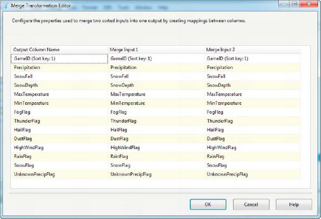
Figure 8-66. Viewing the Merge Transformation Editor
When properly configured, the Merge transformation guarantees that the output will be sorted based on the sort keys.
Merge Join
The Merge Join transformation lets you perform joins on two input datasets, much like SQL joins. The major difference is that unlike SQL Server, which handles data sorting/ordering for you when performing joins, the Merge Join transformation required you to presort your inputs on the join key columns. Figure 8-67 expands the previous Merge transformation example and adds a Merge Join to the input Football Game data.
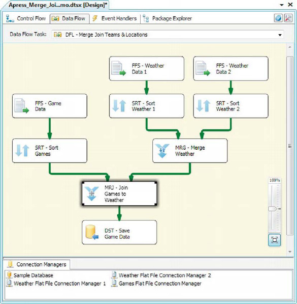
Figure 8-67. Merge Join added to the data flow
The Merge Join Transformation Editor, shown in Figure 8-68, lets you choose the join type. You can select an inner join, left outer join, or full outer join. All of these joins work as you’d expect from working with SQL:
Inner Join returns only rows where the left input key and right input keys match. If there are rows from either input with join key values that don’t match the other input, the rows are not returned.
Left Outer Join returns all the rows from the left input and rows from the right input where the join keys match. If there are rows in the left input that don’t have matching rows in the right input, nulls are returned in the right-hand columns.
Full Outer Join performs all rows from the left and right inputs. Where the join keys don’t match on either the right or left side, nulls are returned in the columns on the other side.
One thing you might notice is that the Merge Join doesn’t support the SQL equivalent of the cross-join or the right outer join. You can simulate the right join by selecting Left Outer Join as the join type and then clicking the Swap Inputs button. This moves your left input to the right, and vice versa. The cross-join could be simulated by adding a derived column to both sides with a constant value in it and then joining on those two columns. The cross-join functionality isn’t as useful, though, except for generating large datasets (for testing purposes, for instance).
In the editor, you can link the join key columns and choose the columns from both sides to return. You can also rename the output columns in the Output Alias list at the bottom of the editor, shown in Figure 8-68.
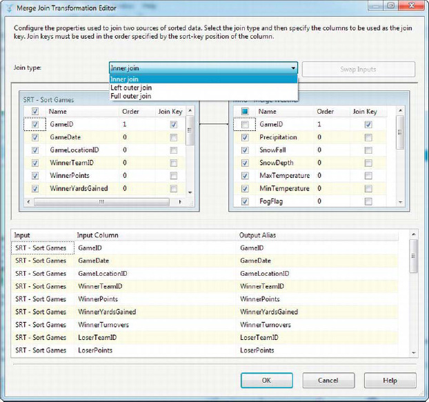
Figure 8-68. Setting attributes in the Merge Join editor
Auditing
SSIS includes a handful of transformations that perform “auditing” functions. Essentially, these tasks allow you to capture metadata about your package or the data flow itself. You can use this metadata to analyze various aspects of your ETL process at a granular level.
Row Count
The Row Count transformation does just what its name says—it counts the rows that pass through it. Row Count sets a variable that you specify to the result of its count. Figure 8-69 shows the Row Count transformation in the data flow.

Figure 8-69. Row Count transformation in the data flow
After you’ve added the Row Count transformation to the data flow, you need to create a variable on the Parameters and Variables tab and add an integer variable to the package, as shown in Figure 8-70. In this case, we’ve chosen to add a variable named RowCount.
![]() NOTE: If you’re not familiar with SSIS variables, don’t fret. We cover them in detail in Chapter 9. For now, it’s just important to know that SSIS variables are named temporary storage locations in memory, as in other programming languages. You can access variables in expressions, which we also discuss in Chapter 9.
NOTE: If you’re not familiar with SSIS variables, don’t fret. We cover them in detail in Chapter 9. For now, it’s just important to know that SSIS variables are named temporary storage locations in memory, as in other programming languages. You can access variables in expressions, which we also discuss in Chapter 9.

Figure 8-70. Adding a variable to the Parameters and Variables tab
The final step in configuring the Row Count transformation is to choose the variable it will transform. You associate the variable with the Row Count transformation by using the VariableName property of the Row Count editor, shown in Figure 8-71.
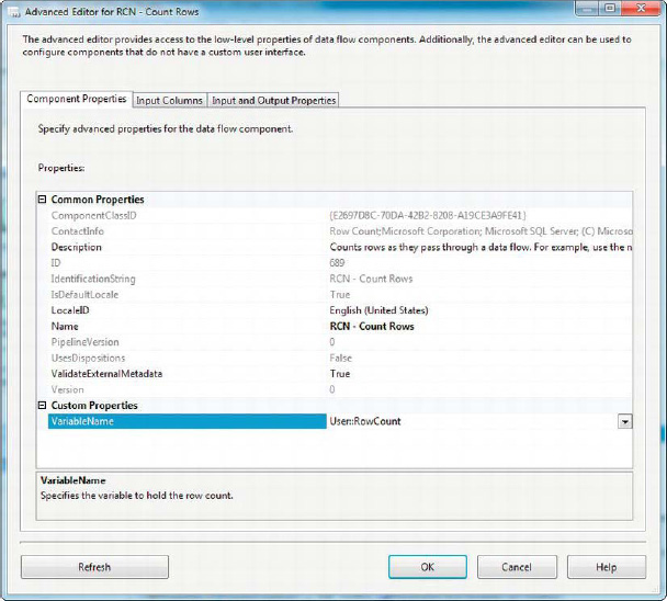
Figure 8-71. Associating a variable with the Row Count transformation
![]() TIP: Don’t try to access the value of the variable set by your Row Count transformation until the data flow is finished. The value is not updated until after the last row has passed through the data flow.
TIP: Don’t try to access the value of the variable set by your Row Count transformation until the data flow is finished. The value is not updated until after the last row has passed through the data flow.
Audit
The Audit transformation gives you a shortcut to add various system variables as columns in your data flow. Figure 8-72 shows the Audit transformation in the data flow.
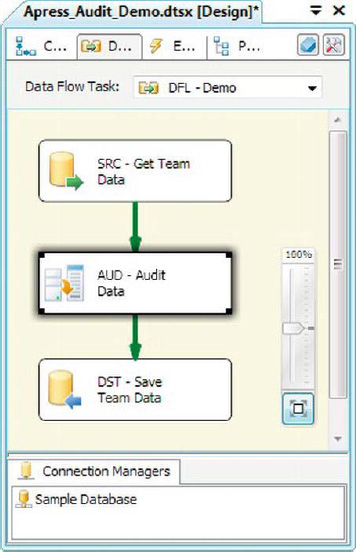
Figure 8-72. Audit transformation in the data flow
After you add the Audit transformation to your data flow, double-click it to edit the properties in the editor. In the editor, you can choose the audit columns to add to your data flow. You can also rename the default output column names. Figure 8-73 shows the audit column selection.

Figure 8-73. Choosing audit columns in the Audit Transformation Editor
![]() TIP: The Audit transformation is a convenience transformation. As an alternative, you can access all of the same system variables and add them to columns in your data flow with the Derived Column transformation.
TIP: The Audit transformation is a convenience transformation. As an alternative, you can access all of the same system variables and add them to columns in your data flow with the Derived Column transformation.
Business Intelligence Transformations
In addition to the transformations covered so far, SSIS provides a handful of Business Intelligence transformations. One of these transformation, the Slowly Changing Dimension transformation, is specific to Dimensional Data ETL. We present this component and efficient alternatives to it in Chapter 17. The remaining components are designed for data scrubbing and validation. We cover these transformations in detail in Chapter 12.
Summary
This chapter presented SSIS data flow transformation components. We talked about the differences between synchronous and asynchronous transformations, as well as blocking, nonblocking, and partially blocking transformations. You looked at the individual transformations you can apply in your data flow, including the wide variety of settings available to each, with examples. The next chapter introduces SSIS variables and the SSIS Expression Language.