C H A P T E R 17
Dimensional Data ETL
We are not in the eighth dimension; we are over New Jersey. Hope is not lost.
—Adventurer Buckaroo Banzai
In the first decade of the 21st century, the terms data warehouse and data mart were suddenly—and without warning—copied and pasted all over every database professional’s résumé. Despite the apparent increased awareness in the professional community, the core components of these structures, dimension and fact tables, remained misunderstood. In this chapter, you’ll look at ways to load data efficiently into your dimensional structures. You’ll begin with an introduction to the terminology and concepts used throughout this chapter.
Introducing Dimensional Data
By now, most database professionals have had some level of exposure to dimensional data. For those who don’t use it every day, this term can be a bit misleading. It doesn’t really refer to any special properties of the data itself, but rather to the dimensional model used to store it. Specifically, dimensional data is stored in dimensional data marts. Data marts are relational databases that adhere to one of two logical structures: the star schema or the snowflake schema. Both of these logical structures consist of two types of tables:
Fact tables contain business measure data, such as sales quantities and dollar amounts.
Dimension tables hold attributes related to the measures stored in the fact tables, such as product colors and customer names.
A star schema features a fact table (or possibly multiple fact tables) related to denormalized dimension tables. Figure 17-1 shows a logical design for a sample star schema that holds sales receipt data for a retail store.

Figure 17-1. Star schema data mart
In a star schema, the dimensions are “flattened out” into denormalized tables. The snowflake schema is a logical structure similar to the star schema, but features normalized, or snowflaked, dimensions. Figure 17-2 features snowflaking of the Time and Geography dimensions from the previous star schema.

Figure 17-2. Data mart with snowflaked dimensions
Because of performance and complexity star schemas are more, but are not always possible to model an OLAP database in such a structure.
Data marts are usually fed by upstream systems such as normalized data warehouses and other databases. The data mart, in turn, is used to feed OLAP databases such as SQL Server Analysis Services cubes or is queried directly for reporting and analysis.
DATA WAREHOUSE, OPERATIONAL DATA STORE, AND OTHER BUZZWORDS
Creating Quick Wins
When your boss says she wants you to optimize an ETL process (or any system for that matter), you can often translate this to mean “tweak it around the edges.” With that in mind, we’ll present some quick changes to give you the biggest bang for the buck.
Run in Optimized Mode
Data Flow tasks in SSIS have a setting called RunInOptimizedMode. Setting this property to True results in the data flow optimizing the task by automatically removing unused columns, outputs, and components from the data flow. In production packages, this property should always be set to True. This should only be set to False when debugging or in very specific troubleshooting scenarios. You can also set RunInOptimizedMode in the SSDT Project Properties. This property setting in SSDT overrides the individual Data Flow task setting when you run the package in SSDT—but only in SSDT. The default package property is False, enabling you to apply the Data Flow property to either True or False. Changing the project property to True will avoid having to update any or all data task properties. Figure 17-3 shows the property page for the Data Flow task.

Figure 17-3. Setting the RunInOptimizedMode property to True
Remove “Dead-End” Components
When debugging SSIS components, it’s common to use the Row Count component in place of a destination for error outputs. In many cases, the value returned by the Row Count is never used. Consider the sample data flow shown in Figure 17-4.

Figure 17-4. Data flow with dead-end components
In this sample data flow, we’re sending the error rows from the Lookup transformations to Row Count transformations. In this case, we aren’t using the values returned by the Row Counts, but SSIS still has to move the unmatched rows down that branch of the data flow and into the components. This is an unnecessary inefficiency in this data flow. Fixing this is as simple as deleting the dead-end Row Counts.
Keep Package Size Small
Owing in large part to the overhead involved in initializing a package, including allocating buffers and automated validations and optimizations, executing a large package can take considerably more time and resources than executing multiple smaller packages to get the same end result. By keeping your packages small, SSIS can execute them more efficiently. There is no hard rule on package size, but SSIS expert Andy Leonard recommends keeping individual packages to a file size of 5 MB or lower. It is also possible to identify common SSIS tasks that run in multiple packages and create smaller packages of these tasks to be used as child packages that can then be called from one or many parent packages. This helps to encapsulate logic and provide reusable components reducing development. This topic is covered in more depth in Chapter 18. Note that by keeping your SSIS packages small, you also gain the benefit of faster loading and validation in SSDT.
Optimize Lookups
There are three main methods of optimizing Lookup transformations in your data flows. The first optimization technique is to use a SQL query to populate your Lookup transformation, instead of the Table or View population mode. The Table or View mode pulls all rows and columns from a table in the database. In many cases, the Lookup transformation doesn’t need all those columns. With the SQL Query mode, you can limit the results to include only a specified list of columns. There’s no point in pulling megabytes (or more) of extraneous data, only to discard it immediately.
The second optimization technique for Lookup transformations involves reusing your Lookup reference data. If you have to perform multiple lookups against the same set of reference data, round-tripping to the database to pull this data two, three, or more times in a single package is a waste of resources. Instead, use the Cache transformation and load that reference data once.
Our third optimization technique for Lookup transformations is to get rid of them. You can do this by performing a join on the server side—in your source query—or by using a Merge Join transformation. Although the Lookup transformation is not technically classified as a blocking transformation, it can actually be worse for performance than a transformation in this group. The issue with the Lookup transformation is that your data flow will not even begin moving data until the Lookup finishes caching its reference data. The Merge Join transformation, which is partially blocking, allows data to move through in a more efficient fashion.
Keep Your Data Moving
The Golden Rule of ETL efficiency is “keep your data moving.” Every second that data is not moving through your data flow is lost processing time that can never be reclaimed. As we discussed in Chapter 15, to keep your data moving, you should minimize the use of blocking transformations and consider performing joins, sorting, and aggregations on the server when possible.
In addition, consider using the SQL Server FAST query hint. By applying the FAST query hint to long-running source queries, SQL Server will send a burst of initial rows to SSIS, allowing your data flow to proceed. Ideally, while those initial rows are winding their way through your data flow, SQL Server will supply more rows to your source component. This hint is particularly useful for long-running queries that feed complex data flows.
![]() TIP: You can find out more about SQL Server query hints at
TIP: You can find out more about SQL Server query hints at http://msdn.microsoft.com/en-us/library/ms181714.aspx.
Minimize Logging
We talked about logging best practices in Chapter 13. The idea is simple: logging processing information requires resources. It takes I/O, network bandwidth, memory, and even a bit of CPU to log. Although you don’t want to eliminate logging completely, you should target your production logging settings to record the minimal amount of information you need to monitor and troubleshoot your ETL processes.
Use the Fast Load Option
We discussed the fast load and bulk insert options available for OLE DB and SQL Server destination adapters in Chapter 7. When inserting rows into SQL Server tables, use these options when possible. The fast load options are much more efficient than individual, one-row-at-a-time round-trips to the server.
Understanding Slowly Changing Dimensions
Slowly changing dimensions (SCDs) are the physical implementation of the dimensions we discussed earlier in this chapter. Basically, SCDs put the dimensional in your dimensional data. SCDs are divided into four major types, which we discuss in the following sections.
Type 0 Dimensions
Type 0 dimensions, also known as nonchanging dimensions or very slowly changing dimensions come in two flavors:
- Dimensions with attributes that never change (such as a Gender dimension)
- Dimensions with attributes that very rarely change (such as a US States dimension)
Type 0 dimensions are generally populated one time with load scripts. The occasional update to these dimensions is usually just an operation that adds records, which can also be performed with one-off scripts. As an example, consider a Date dimension with 10 years’ worth of dates in it. You might need to add another 10 years’ worth of date attributes to the dimension, but this doesn’t affect the existing entries. With this in mind, our best advice for Type 0 dimensions is to populate them and update them as necessary with static one-off scripts.
Type 1 Dimensions
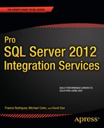
Apart from nonchanging dimensions, Type 1 SCDs are the simplest type of dimension to implement—they have no requirement to store historical attribute values. When attributes in a Type 1 SCD change, you simply overwrite the old ones with the new values. A standard Type 1 SCD implementation involves storing a surrogate key (the IDENTITY column in SQL Server serves this purpose well, as will using a SEQUENCE that is introduced in SQL 2012), the business key for the inbound dimension attributes, and the dimension attribute values themselves. Consider the DimProduct Type 1 SCD table shown in Figure 17-5.
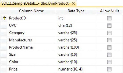
Figure 17-5. DimProduct type 1 dimension table
The DimProduct table holds entries describing all the products. In this example, the ProductID is the surrogate key, UPC is the business key, and the remaining columns hold the attribute values. The update pattern for the Type 1 SCD is simple, as shown in the flowchart in Figure 17-6.
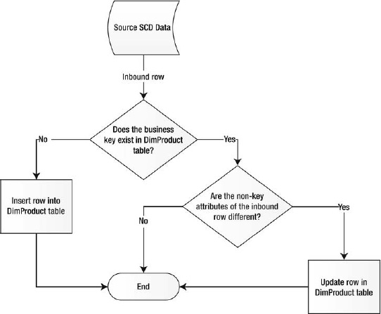
Figure 17-6. Type 1 SCD update flowchart
The process for updating the Type 1 SCD is a simple upsert (update-or-insert) operation based on the business key. If the business key of the inbound row exists in the dimension table, it’s updated; if the key doesn’t exist, it’s inserted. There are several ways to implement Type 1 SCD updates:
- You can build out your own data flow by hand, which will perform the necessary comparisons and individual updates and inserts.
- You can create an SSIS custom component, or use a prebuilt custom component, to do the hard work for you.
- You can insert the raw data into a staging table and follow up with a set-based
MERGEinto the dimension table.- You can use the SSIS Slowly Changing Dimension Wizard to build out your SCD update data flow.
The main question you need to answer when deciding which method to use is, where can you perform the necessary dimension member comparisons most efficiently—in the data flow or on the server? In general, the most efficient comparisons can be performed on the SQL Server side.
With that in mind, we’ll skip building out a data flow by hand as it tends to be the most inefficient and error-prone method. If you’re interested in pursuing this option, we recommend using the Slowly Changing Dimension Wizard instead to build out a prototype. This will give you a better understanding of how the data flow can be used to update your SCD. We’ll consider the Slowly Changing Dimension Wizard later in this section.
Using a prebuilt SSIS custom component (or building your own) is another viable option, but it’s outside the scope of this chapter. We recommend looking at some of the samples on CodePlex (www.codeplex.com) to understand how these components work.
Our preferred method (without custom components) is loading your dimensions into a staging table and performing the dimension updates on the server directly. Set-based updates are the most efficient method of updating dimensional data. The control flow in Figure 17-7 shows the basic layout of the Type 1 SCD set-based update.
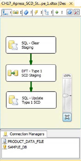
Figure 17-7. Set-based Type 1 SCD update package
The first step of the process is to truncate the staging table with an Execute SQL task:
TRUNCATE TABLE Staging.DimProduct;
The next step is the data flow, which simply moves the Product dimension data from the source to the staging table, as shown in Figure 17-8.

Figure 17-8. Data flow to load the staging table
The Flat File Source pulls the Product dimension from a flat file, and the OLE DB Destination pushes the data to the staging table. In between, there’s an additional step that generates an SHA1 hash code for each row of data as it moves through the data flow.
HASH CODES
The .NET code we use to generate a hash code is very efficient, utilizing MemoryStream and BinaryWriter, as shown in the following code snippet.
public class ScriptMain : UserComponent

{


  MemoryStream ms;

  BinaryWriter bw;

  SHA1Managed sha1;


  public override void PreExecute()

  {

    base.PreExecute();

    sha1 = new SHA1Managed();

  }


  public override void PostExecute()

  {

    base.PostExecute();

  }


  public override void Input0_ProcessInputRow(Input0Buffer Row)

  {

    ms = new MemoryStream();

    bw = new BinaryWriter(ms);

    if (Row.UPC_IsNull)

    {

      bw.Write((Int32)0);

      bw.Write((byte)255);

    }

    else

    {

      bw.Write(Row.UPC.Length);

      bw.Write(Row.UPC);

    }

    bw.Write('|'),


    // ...Write additional columns to BinaryWriter


    byte[] hash = sha1.ComputeHash(ms.ToArray());

    Row.Hash = hash;

    ms.Dispose();

    bw.Dispose();

  }
All the columns are written to BinaryWriter with the length of the column followed by the value. In the case of a NULL value, a length of zero is written, followed by a single byte value (this is a value that can’t be generated in inbound data). Each column is followed by a vertical bar separator character. The concatenated binary string is then fed into an SHA1 generation function, and the output is assigned to the Hash column.
The final step of the Type 1 SCD update is a single update-or-insert (upsert) operation from the staging table to the dimension table. The T-SQL MERGE statement is perfectly suited for this job. The MERGE statement lets you perform UPDATE and INSERT operations in a single statement, as shown here:
MERGE INTO dbo.DimProduct AS Target

USING Staging.DimProduct AS Source

  ON Target.UPC = Source.UPC

WHEN MATCHED AND Target.Hash <> Source.Hash

THEN UPDATE SET Target.Category = Source.Category,

  Target.Manufacturer = Source.Manufacturer,

  Target.ProductName = Source.ProductName,

  Target.Size = Source.Size,

  Target.Price = Source.Price,

  Target.Hash = Source.Hash

WHEN NOT MATCHED

THEN INSERT (UPC, Category, Manufacturer, ProductName, Size, Price, Hash)

  VALUES (Source.UPC, Source.Category, Source.Manufacturer, Source.ProductName, Source.Size,

    Source.Price, Source.Hash);
![]() NOTE:
NOTE: MERGE provides a means to incorporate INSERT, UPDATE, and DELETE in one statement. However, separating these steps into individual statements can improve overall performance. Compare the costs of both methods to ensure that the most efficient query is used.
The notable shortcoming of a Type 1 SCD is that historical values will be lost to an update of the current value. However, the update process is easier than a Type 2 or Type 3 SCD and also uses less space, as long-term history is not maintained.
Type 2 Dimensions
Because they maintain a long-term history of attribute values, Type 2 dimensions are slightly more complex to manage than Type 1 dimensions. The schema of a Type 2 SCD table differs from a Type 1 SCD in that it can contain up to three extra columns to denote a current or historic version. The additional column(s) allow the dimension table to contain the historic values rather than overwriting the affected column(s) with the current value. The dimension could contain a single column that indicates whether the row has the most current value, as displayed in Figure 17-9.
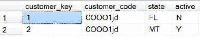
Figure 17-9. Type 2 SCD result set
While new or updated values are always inserted into Type 2 dimensions, there are additional flags on existing rows that must also be updated, such as the effective date, end date, or active column. Adding a column to indicate only whether the row is the most current enables you to ensure that all historic changes are kept, but not to define when the specific row was active. The addition of both an active column and an end-date column would provide the means of maintaining historic values that can then be associated with the proper time frame.
The Active column denotes whether the row holds the current value, but lacks the ability to track when the value(s) were in effect. The dimension table could include a start- and end-date column, which could maintain the historic values and times, when the end date is NULL this represents the current value, or an effective date column and a column representing active or historic. The process of updating a Type 2 SCD is shown in Figure 17-10.

Figure 17-10. Type 2 SCD update flow
SSIS provides a Data Transformation task that can be used for both Type 1 and Type 2 SCDs. The first step in using the SCD transformation task for a Type 2 SCD is to decide whether you are going to track changes in your table by either using a simple indicator to identify current and expired records, or using effective dates. The component doesn’t natively allow you to use both, although you can customize the output to do so. Figure 17-11 demonstrates using a SCD transformation task in a data flow.

Figure 17-11. SSIS slowly changing dimension component
Type 3 Dimensions
A Type 3 SCD tracks changes by using separate columns, which limits the history to the number of columns that can be added to the dimension table. This obviously provides limitations, and the dimension table will begin to look more like a Microsoft Excel spreadsheet, as shown in Figure 17-12.
Figure 17-12. Query results of a Type 3 SCD
There are several complexities in implementing a Type 3 SCD—first and foremost modifying the table schema for each update, which make this a less than desirable means of tracking historic attributes, As a Type 3 SCD is limiting and requires changing the schema of the dimension table, it is not supported in the SCD Transformation task. It is possible to use an Execute SQL task to automate updating a Type 3 SCD, but if at any point the dimension table was referenced in a Data Flow task, it would fail the validation phase based on the schema change. The issues don’t end with the processing of the dimension, but also include using the dimension in an SSAS cube or for a report, again as based on the ever-changing schema. Although utilizing a Type 3 SCD is an option, utilizing a Type 1 or 2 SCD is preferable.
Summary
This chapter introduced several tools and methods for optimizing your SSIS packages. Many of these optimizations rely on performing operations at the source when possible and limiting the data pulled through the ETL process. We also discussed the different types of dimensions and outlined ways that each dimension could be updated. In the next chapter, we’ll consider the powerful SSIS parent-child design pattern.