C H A P T E R 7
Source and Destination Adapters
“All rivers flow into the sea, yet the sea is not full.”
—King Solomon
In SSIS, the data flow is your primary tool for moving data from point A to point B and manipulating it along the way. The data flow is a powerful concept that allows you to encapsulate your data movement and transformation as a self-contained task of the control flow. The data flow moves your data from a source to a destination, like King Solomon’s river moves water from its source to the sea. This chapter introduces the data flow and discusses data flow source adapters, destination adapters, and the new Source and Destination Assistants.
The Data Flow
The data flow is contained within the confines of the Data Flow task, which itself exists in the control flow. The Data Flow task is shown in Figure 7-1.
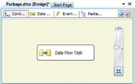
Figure 7-1. The Data Flow task on the BIDS designer surface
You add a Data Flow Task to the control flow by dragging and dropping it from the SSIS Toolbox over to the BIDS designer surface. Because the Data Flow Task is a control flow task, the data flow represents a powerful self-contained subset of the control flow. The purpose of having a data flow is to separate data movement and manipulation—the primary purpose of ETL—from work flow management. As you can see in Figure 7-2, any given data flow can be fairly complex. You can also include multiple Data Flow tasks in a single control flow. We cover the sources, destinations, and transformations shown in the sample data flow, and many more, in this chapter and the next.

Figure 7-2. Data flow consisting of several data flow components
The components that make up the data flow can be divided into three categories: source adapters that pull data into the data flow; transformations that allow you to manipulate, modify, and direct your data; and destination adapters that allow you to push data out of the data flow to persistent storage or into other systems for further processing. In this chapter, we consider the sources and destinations that SSIS provides to pull data into and push data out of your data flows.
Technically speaking, all data flow components derive from a single base class called the PipelineComponent class. This class exposes properties such as BufferManager, which provides access to the two-dimensional storage object (that is to say, a tabular rowset) holding your data as it moves through the data flow. The PipelineComponent class also has methods such as AcquireConnection, which establishes connectivity to your data sources via connection managers. In the out-of-the-box stock components we discuss in this chapter, these properties and methods are already fully developed for you, so you don’t have to deal with them directly.
![]() NOTE: We discuss the details of the
NOTE: We discuss the details of the PipelineComponent class and developing your own custom components in depth in Chapter 22.
Sources and Destinations
In the SSIS data flow, source adapters are components that pull data from well-defined data stores. Source adapters use connection managers to connect to, and pull data from, databases such as SQL Server and Oracle, flat files, XML, or just about any other source you can define. Destination adapters are the opposite of source adapters—they push data to data stores. Destination adapters use connection managers to send data to databases, flat files, Excel spreadsheets, or any other destination you can connect to.
Although you can create extremely complex data flows in SSIS, the simplest useful data flow you can create might consist of a single source adapter connected to a single destination adapter. For this example, let’s consider a simple data flow that extracts data from a flat file and loads it into a SQL Server database table. This is considered straight pull, in that no transformations are applied to the data as it moves from source to destination. For the purposes of this chapter, assume you’re editing a brand new SSIS package in BIDS with a single data flow.
Source Assistant
The Source Assistant is new to SQL Server 11 SSIS. When you drag this component from the SSIS Toolbox to the designer surface, BIDS opens the Add New Source dialog box. This dialog asks you to choose a type of source and a connection manager to use. As you can see in Figure 7-3, the source assistant window lets you choose from several types of sources. For our simple data flow sample, we’ve selected a Flat File source type and a <New> connection manager.
![]() NOTE: The Show Installed Only check box limits the types shown to only those that are installed on your local development machine.
NOTE: The Show Installed Only check box limits the types shown to only those that are installed on your local development machine.

Figure 7-3. Add New Source dialog box of the Source Assistant
When you choose the <New> connection manager, the Connection Manager Editor pops up. The editor is specific to the type of connection manager you want to create—the Flat File Connection Manager Editor has different properties from the SQL Server Connection Manager Editor. The Flat File Connection Manager Editor is shown in Figure 7-4.
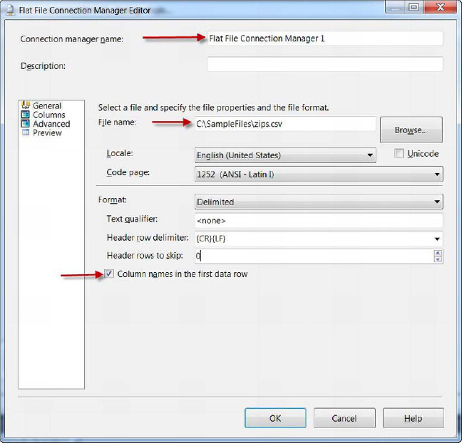
Figure 7-4. Flat File Connection Manager Editor’s General properties
We’ll choose the Flat File source and <New> connection manager from the Add New Source dialog box. Then we use the Flat File Connection Manager Editor to set the properties for the flat file and select a source file. As you can see in Figure 7-4, we chose a comma-delimited file named zips.csv, updated the connection manager name, and selected the Column Names in the First Data Row check box on the General page. We left the Locale, Code Page, and other options at their default values.
On the Columns page of the editor, you have two options for flat files. You can change the row delimiter, which is the character or combination of characters that ends each line of the flat file, and you can change the column delimiter, which is the character or character combination that separates fields in the file. In this case, we’ve chosen the default {CR}{LF} (carriage return/line feed) combination for the row delimiter, and the Comma (,) for the column delimiter for .csv files. The Columns page also gives you a preview of the source data. Figure 7-5 highlights these options on the Columns page of the editor.
![]() NOTE: The {CR}{LF} combination is a common row delimiter for Windows text files. Files generated on some other operating systems, such as Unix, use only the {LF} character as row delimiters. Keep this in mind when dealing with flat files generated by non-Windows systems.
NOTE: The {CR}{LF} combination is a common row delimiter for Windows text files. Files generated on some other operating systems, such as Unix, use only the {LF} character as row delimiters. Keep this in mind when dealing with flat files generated by non-Windows systems.
Figure 7-5. Editing properties in the Columns page of the Flat File Connection Manager Editor
The Advanced page is the third page of the editor. On this page, you can change column-specific properties for your data source. You can change the ColumnDelimiter property for individual columns, so that one or more columns can have a special delimiter (useful if you have a single input column that needs to be split in two, for instance). You can also change the DataType for the column (default is string, or DT_STR) and the output column width (default is 50 for string). There are additional properties for DataPrecision and DataScale, which determine the number of total digits in a numeric (DT_NUMERIC) column and the number of digits after the decimal point, respectively. Figure 7-6 shows the Advanced page of the Flat File Connection Manager Editor.
For our sample columns, properties were set as shown in Table 7-1.
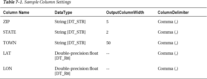
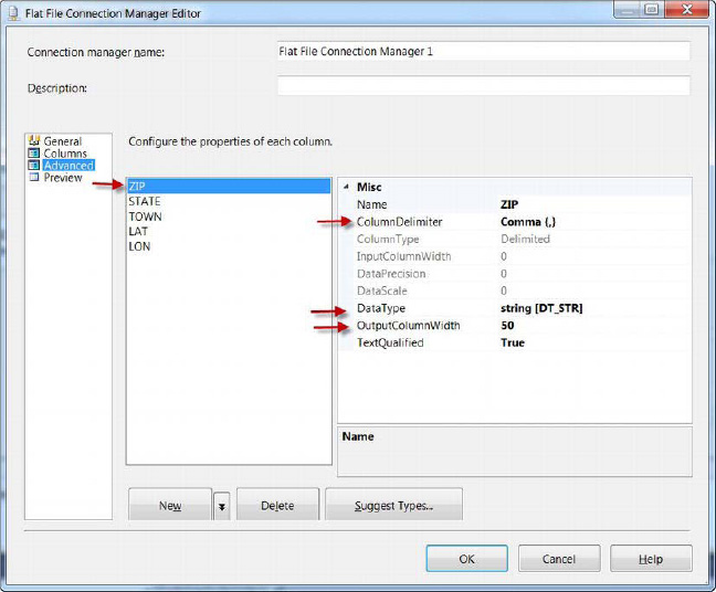
Figure 7-6. Editing column properties in the Advanced page of the Flat File Connection Manager Editor
PRECISION AND SCALE
After you configure the connection manager, the Source Assistant adds the appropriate type of source adapter to your data flow, as shown in Figure 7-7. The Flat File Connection Manager you created appears in the Connection Managers tab of the BIDS designer.

Figure 7-7. Flat File source adapter created by the Source Assistant
Destination Assistant
In addition to the new Source Assistant, SQL Server 11 SSIS also includes a new Destination Assistant. Whereas the Source Assistant guides you through adding source adapters to data flow, the Destination Assistant walks you through adding destination adapters. Just drag the Destination Assistant to the designer surface, and the Add New Destination dialog box, shown in Figure 7-8, appears. As in the Source Assistant dialog box, you can choose a type and connection manager for your new destination. You can also toggle the Show Installed Only check box to list only currently installed destination types or all supported types.
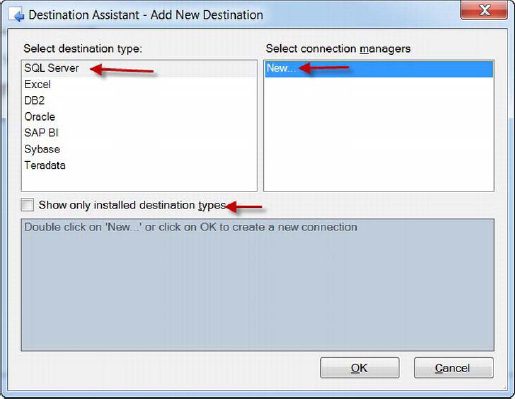
Figure 7-8. Add New Destination dialog box of the Destination Assistant
For this example, we chose the SQL Server destination type and <New> connection manager. The SQL Server destination type presents us with the OLE DB Connection Manager Editor, with the Native OLE DBSQL Server Native Client 11.0 provider selected. This editor allows you to choose the server name, provide authentication credentials, and choose the database to log into, as shown in Figure 7-9.

Figure 7-9. Configuring the OLE DB Connection Manager
After you edit the connection manager properties, BIDS adds the appropriate destination adapter to your data flow, in this case an OLE DB destination. If there is a red x on the destination adapter, as shown in Figure 7-10, it means you need to configure additional properties of the destination adapter. In this case, we need to drag the green Flat File source adapter output path arrow and connect it to the OLE DB destination adapter and configure the destination adapter’s properties to point it at a table in a database.
![]() NOTE: The OLE DB Connection Manager created by the Destination Assistant has a default name of the form
NOTE: The OLE DB Connection Manager created by the Destination Assistant has a default name of the form server_name.database_name. You will probably want to change this to a friendlier name. Just right-click the connection manager in the Connection Managers tab and choose Rename from the context menu. In our example, we renamed the database connection manager to Source_DB.
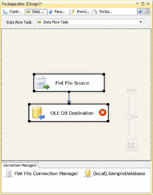
Figure 7-10. OLE DB destination adapter created by the Destination Assistant
After connecting the Flat File source adapter to the OLE DB destination adapter, we still need to configure the OLE DB destination adapter. By double-clicking the OLE DB destination adapter, we can pull up the OLE DB Destination Editor. With this editor, we chose the OLE DB Connection Manager, the data access mode, and the name of the target table. We chose Table or View – Fast Load as the data access mode, which lets us also set the Rows per Batch and Maximum Insert Commit Size options. We changed these from the default values. These options are shown in Figure 7-11.

Figure 7-11. Setting properties for OLE DB destination in the editor
The Mappings page of the editor gives you the opportunity to map the destination component’s input columns to its output columns. When you connect the destination adapter to the data flow, BIDS tries to automatically map the columns based on name. In our example, all of the columns in the source file have the same names as the columns in the target table, so the mapping is performed for us automatically. If you need to map an input column to a differently named output column, you can change the mappings by connecting them in the upper portion of the mapping window or by changing them in the grid view in the lower portion of the screen, as shown in Figure 7-12.

Figure 7-12. Mapping page of the OLE DB destination editor
After you’ve completed the destination configuration, the red x will disappear from the component in the data flow designer in BIDS. Running the package in BIDS shows that 29,470 rows are imported from the flat file to the database table, as you can see in Figure 7-13.
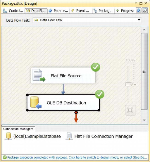
Figure 7-13. Successful execution of the simple data flow created with Source and Destination Assistants
Database Sources and Destinations
In the previous sections, we showed you how to use the Source and Destination Assistants to set up a simple package to pull data out of a flat file and push it into a database. We chose to demonstrate with the Flat File source and OLE DB destination adapters because their use is a very common scenario, especially when using SSIS to pull data from legacy systems for which no direct connection is available and push it into a SQL Server database. This section details database sources and destinations and shows you how to configure their more-advanced features.
OLE DB
OLE DB source and destination adapters allow you to connect to a variety of OLE DB data stores, but they are commonly used for database connectivity because they provide good performance and support a wide variety of relational databases. For this example, we’ll configure an OLE DB source adapter and OLE DB destination adapter to both connect to a SQL Server instance and move data from one table to another. This will be a very simple demonstration, but will give you an opportunity to uncover a wide range of OLE DB configuration options.
For our example, we have two tables: one named LastName, containing a list of the most common surnames in the United States (data obtained from US Census Bureau), and one called LastName_Stage that we’ll copy the surnames to.
Our first step was to create two connection managers named Source_DB and Dest_DB, respectively. These two connection managers point at the same server and database in the example, but in the real world they would likely point at different servers or different databases on the same server. This is why we created two separate connection managers for them. Table 7-2 shows the variety of options you can choose in the OLE DB Source Editor, which is pictured in Figure 7-14.
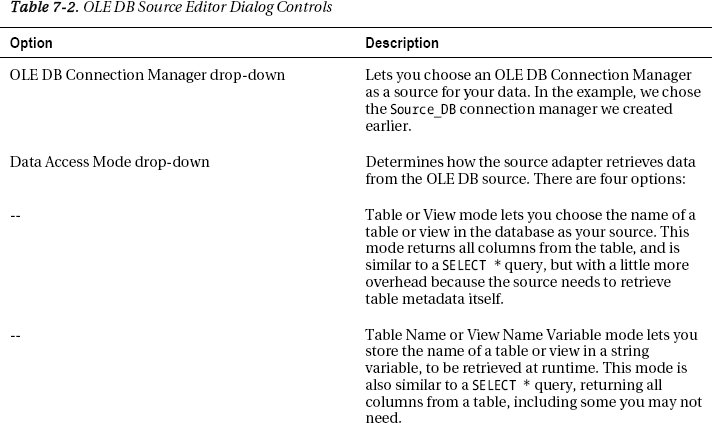
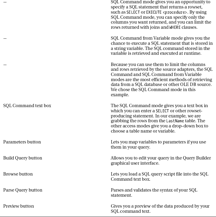
![]() NOTE: It’s a best practice to use SQL
NOTE: It’s a best practice to use SQL SELECT statements when pulling data from source tables for a couple of reasons. First, your table may have more columns than you actually need to pull. It’s a good idea to minimize the amount of data you pull into your data source for efficiency reasons. Second, the Table or View access mode incurs additional overhead that is avoided with the SQL Command or SQL Command from Variable access mode.
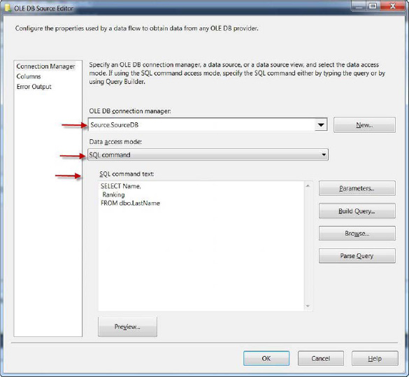
Figure 7-14. Configuring the OLE DB source to pull data from the LastName table
In the OLE DB source, we’ve used an OLE DB parameterized query. In a parameterized query, you define parameters and map variables to those parameters. At query execution time, both the parameterized query and the parameter values are passed on to the server. The server executes the query with the appropriate values in place of the parameters. In our example, we’ve used the following simple query:
In OLE DB the ? is used as a parameter placeholder. Parameters in OLE DB are indicated by their ordinal position (the order in which they appear in the query). The first parameter is Parameter0, the second is Parameter1, and so on. Clicking the Parameters button on the editor dialog gives you the Set Query Parameters dialog box. In this window, you can map variables to parameters, as shown in Figure 7-15.
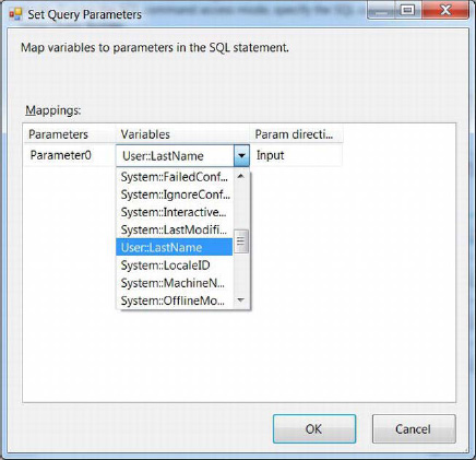
Figure 7-15. Mapping a variable to an OLE DB parameter in our sample source query
We created a string variable named User::LastName and populated it with a SQL wildcard LIKE operator pattern (in this case, we chose [A-M]%, which will return all names that start with the letters A through M). Figure 7-16 shows the Variables portion of the Parameters and Variables window, where we defined the User::LastName variable.
![]() NOTE: For a detailed discussion of creating and using SSIS variables, see Chapter 9.
NOTE: For a detailed discussion of creating and using SSIS variables, see Chapter 9.
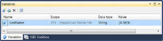
Figure 7-16. Defining a variable in the Variables portion of the Parameters and Variables window
The next step in our sample is configuring the OLE DB destination, as shown in Figure 7-17.
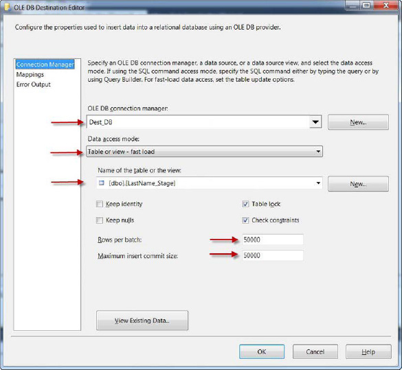
Figure 7-17. Configuring the OLE DB Destination Editor to output to a table
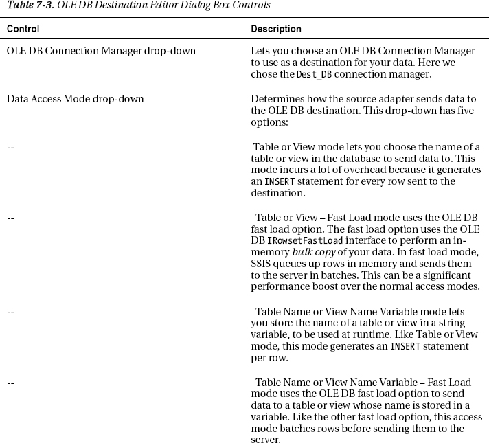
With the OLE DB Destination Editor, you can configure exactly where your data is going as well as some of the properties that determine how that data gets there. Table 7-3 is a breakdown of the OLE DB Destination Editor.

![]() NOTE: Generally we set Rows per Batch and Maximum Insert Commit Size to a value between 50000 and 100000. We recommend setting these values to something other than the defaults. Setting these to nondefault values will help the provider optimize its memory usage and avoid some issues reported with older versions of some OLE DB providers.
NOTE: Generally we set Rows per Batch and Maximum Insert Commit Size to a value between 50000 and 100000. We recommend setting these values to something other than the defaults. Setting these to nondefault values will help the provider optimize its memory usage and avoid some issues reported with older versions of some OLE DB providers.
A successful run of this package results in a screen like the one shown in Figure 7-18.

Figure 7-18. Successful OLE DB source to OLE DB destination package execution
ADO.NET
The ADO.NET source and destination adapters allow you to create managed .NET SqlClient connections. Because they are managed code, these types of connections tend to provide weaker performance than their native-mode OLE DB counterparts overall. On the other hand, they are easier to access and manage programmatically from within .NET code, such as Script tasks and script components, precisely because they are managed. In many cases, particularly when small numbers of rows are involved, the performance difference between ADO.NET and OLE DB source and destination adapters is negligible.
The ADO.NET source adapter has a simplified interface that allows you to choose an ADO.NET connection manager and one of two access modes: Table or View mode or SQL Command mode. Unlike the OLE DB source adapter, parameters are not supported with the ADO.NET source adapter.
![]() TIP: Although you can’t parameterize an ADO.NET source adapter, you can set the
TIP: Although you can’t parameterize an ADO.NET source adapter, you can set the SqlCommand property for the component to an expression. You can access this property via the Data Flow task properties. We discuss SSIS expressions in detail in Chapter 9.
The ADO.NET destination adapter also has a simple interface. It allows you to choose an ADO.NET Connection Manager and a table or view to send output to. There is an additional check box to Use Bulk Insert When Possible, which will take advantage of memory-based bulk copy, similar to the OLE DB IRowsetFastLoad interface.
SQL Server Destination
The SQL Server destination adapter provides high-speed bulk insert, similar to the Bulk Insert task. The main difference is that, unlike the Bulk Insert task that sits in the control flow, the SQL Server destination sits at the end of a data flow—so you can transform your data prior to bulk loading it. Another difference is that the SQL Server destination doesn’t read its source data from a file. Instead it bulk loads from shared memory, which means you can’t use it to load data to a remote server.
SQL Server Compact
SSIS has a SQL Server Compact destination adapter that lets you send data to a SQL Server Compact Edition (CE) instance. One thing to keep in mind when connecting to SQL Server CE is that only a 32-bit driver is available.
Files
Flat files and databases are arguably the most common sources and destinations used in SSIS packages, which is why we started this chapter with a detailed discussion of these two classes of adapters. However, there are still more file-based sources and destinations available. We discuss these source and destination adapters, and their properties, in this section.
Flat Files
When you’re talking about importing and exporting files, odds are very high you’re talking about flat files. Because they’re so prevalent, it’s no surprise that SSIS provides extensive support and options for importing data from and exporting data to flat files. When we talk about flat files, we’re talking about delimited files, fixed-width files, and ragged-right files, which are files with fixed width-columns, except for the very last column, which can be of varying length.
We demonstrated a simple flat-file import in the first sample in this chapter, and now we’ll circle back to discuss the advanced options with another example. We started by creating and configuring a Flat File Connection Manager and an ADO.NET Connection Manager in a new package. We configured the Flat File Connection Manager as shown in Figure 7-19.

Figure 7-19. Configuring the Flat File Connection Manager
We configured the Flat File Connection Manager to pull data from a delimited file named states.txt. The file holds Unicode data, so we selected the Unicode check box. Because we’re using Unicode, the Code Page drop-down is disabled because it is irrelevant. The format is delimited using a pipe delimiter for most columns—more on this later; and finally, the file has the column names in the first row.
We also tweaked some settings on the Advanced page of the Flat File Connection Manager Editor. We set the ColumnDelimiter, which tells SSIS how to divide your file into columns, to the pipe character (|) for most of the columns. In the last field of the file, we have the Longitude and Latitude of each state capital, separated by a comma (,), as shown in Figure 7-20. So really we have what’s known as a mixed-delimiter file.
When you create the flat file connection, all columns default to 50-character strings. In our case, we adjusted the DataType setting on some of the columns: we changed the Long and Lat columns to the double-precision float [DT_R8] data type, for instance.

Figure 7-20. Adjusting column-level settings on the Advanced page of the Flat File Connection Manager Editor
![]() NOTE: We’re just giving a brief overview of the Flat File Connection Manager in this section. We discussed the connection managers and their configurations in detail in Chapter 4.
NOTE: We’re just giving a brief overview of the Flat File Connection Manager in this section. We discussed the connection managers and their configurations in detail in Chapter 4.
After we configured the Flat File Connection Manager, we configured the Flat File source adapter to use it. Although the Flat File source adapter has a standard, simplified editor, we chose to configure this component by using the Advanced Editor that all components have by default. To access the Advanced Editor, shown in Figure 7-21, simply right-click the Flat File source adapter and choose Show Advanced Editor from the context menu.
The first option we set, on the Connection Managers tab of the Advanced Editor, was to tell the Flat File source adapter to use the Flat File Connection Manager.

Figure 7-21. Configuring the Flat File source adapter to use the Flat File Connection Manager
The Column Mappings tab maps the external columns (which are the columns defined by the connection manager) and the output columns (which are the columns that are output by the Flat File source adapter). You can change column mappings in the top portion of the window by dragging and dropping external columns over to the Output Columns box, or you can change them in the lower portion of the window by choosing different columns from the drop-down lists in the grid box. The Column Mappings tab is shown in Figure 7-22.

Figure 7-22. Mapping columns in the Advanced Editor
The Input and Output Properties tab gives you access to advanced column-level metadata. In this view, you can see the individual external columns, output columns, and their properties, as shown in Figure 7-23.
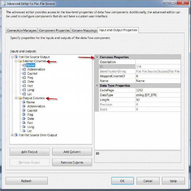
Figure 7-23. Reviewing column-level metadata in the Input and Output Properties tab
After configuring the Flat File source adapter, we connected its output to the ADO.NET destination, and configured the ADO.NET destination adapter to use the ADO.NET Connection Manager. The source-to-destination connection and ADO.NET destination adapter are shown in Figure 7-24 and Figure 7-25.

Figure 7-24. Connecting the Flat File source adapter output to the ADO.NET destination adapter input
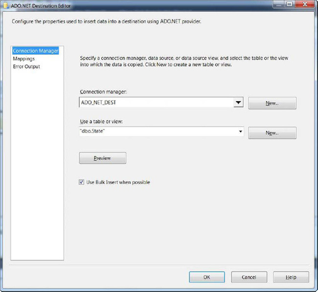
Figure 7-25. Configuring the ADO.NET destination adapter
The Flat File destination adapter is the opposite of the Flat File source adapter. Instead of pulling in the contents of a flat file and outputting the data into your data flow, the Flat File destination adapter accepts the input from your data flow and outputs it to a flat file.
Excel Files
Business users often use spreadsheets as ad hoc databases. From a business user’s perspective, it makes sense because they, and all their colleagues, are familiar with the spreadsheet paradigm. They all understand the user interface, how to implement simple and even complex calculations, and how to format the interface exactly as they want it. From the IT perspective that developers and DBAs bring to the table, there are few things scarier than the thought of hundreds of gigabytes of business information floating around the aether, possibly unsecured, in ad hoc spreadsheet formats.
The Excel source and destination can help you pull data out of spreadsheets and store it in secure, structured databases, or extract data from well-defined systems and put it in a format your business users can easily manipulate.
For this example, we’ll assume a simple package with two data flows in it. One data flow will read the contents of an Excel spreadsheet and store it in a table, and the second will read the contents of that same table and output it to an Excel spreadsheet. Our sample Excel spreadsheet looks like Figure 7-26.
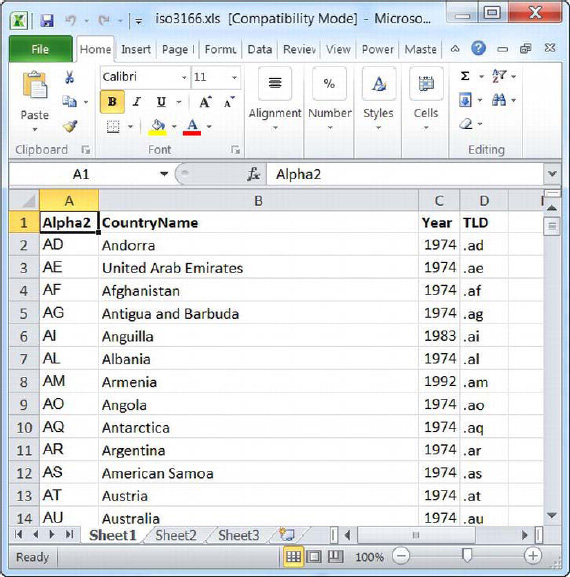
Figure 7-26. Source Excel spreadsheet containing ISO 3166 country codes and names
The first step is to create an Excel Connection Manager. Right-click in the Connection Managers tab and choose New Connection. Then choose the EXCEL connection manager type. You’ll be presented with the Excel Connection Manager dialog box, shown in Figure 7-27. In this example, we chose an Excel file named iso3166.xls with a list of country names and abbreviations from the ISO 3166 standard, we selected Microsoft Excel 97–2003 format, and we selected the check box indicating that the first row of data on the spreadsheet holds the column names.
![]() NOTE: ISO 3166 is the international standard for country codes and names. Whenever possible, it’s a good idea to use recognized standards instead of reinventing the wheel.
NOTE: ISO 3166 is the international standard for country codes and names. Whenever possible, it’s a good idea to use recognized standards instead of reinventing the wheel.
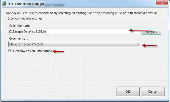
Figure 7-27. Setting Excel Connection Manager properties in the editor dialog box
We also created an OLE DB Connection Manager, as described in the “Destination Assistant” section of this chapter.
The next step is to drag the Excel source adapter and OLE DB destination adapter onto the BIDS designer surface and connect them. We then edited the Excel source by double-clicking it to pull up the Excel Source Editor. In the editor, we chose the Excel Connection Manager we just created, chose a data access mode of Table or View, and selected the first spreadsheet in the Excel workbook, named Sheet1$, as you can see in Figure 7-28.
![]() NOTE: The Excel Source Editor lets you choose entire worksheets or named ranges of cells from an Excel workbook.
NOTE: The Excel Source Editor lets you choose entire worksheets or named ranges of cells from an Excel workbook.

Figure 7-28. Configuring the Excel source in the editor
You can look at the source columns by selecting the Columns tab of the Excel Source Editor. The Columns page gives you a list of available external columns (the columns in the physical Excel file) with a check box next to each one. You can deselect a given column if you don’t want it included in your data flow. Figure 7-29 shows the Columns page of the Excel Source Editor.

Figure 7-29. Viewing the Columns page of the Excel Source Editor
As an alternative to choosing the Table or View access mode and selecting a worksheet name, you can choose SQL Command mode and enter a SQL-style query to get the same data from your Excel spreadsheet. The following query retrieves the same data from your worksheet that we’re grabbing in the current example:
SELECT Alpha2,

    CountryName,

    Year,

    TLD

FROM [Sheet1$];
![]() NOTE: The Excel source and Excel destination adapters use the Microsoft OLE DB Provider for Jet 4.0 and the Excel Indexed Sequential Access Method (ISAM) driver to read from and write to Excel spreadsheets. Bear in mind that this driver provides a very limited subset of SQL-style query syntax, and it does not support many T-SQL features you may be used to.
NOTE: The Excel source and Excel destination adapters use the Microsoft OLE DB Provider for Jet 4.0 and the Excel Indexed Sequential Access Method (ISAM) driver to read from and write to Excel spreadsheets. Bear in mind that this driver provides a very limited subset of SQL-style query syntax, and it does not support many T-SQL features you may be used to.
When you set up an Excel source adapter, it tries to automatically determine the data types of the external columns by sampling the data in the spreadsheet. There is currently no way to force or coerce the data type of an Excel column to a more appropriate type, apart from modifying the data in your spreadsheet. Table 7-4 shows all of the data types supported by the Excel ISAM driver.

If SSIS overestimates the size or data type of your Excel columns—for instance, (nvarchar(255) for an nvarchar(2) column—you may need to add a Derived Column transformation (which we cover in the next chapter) to your data flow to convert your columns to the appropriate types. To complete the data flow, we simply configured the OLE DB destination to point at a database table and mapped the columns as we described in the “Destination Assistant” section of this chapter. A successful run of this sample package looks like Figure 7-30.
JET DRIVERS AND 64-BIT
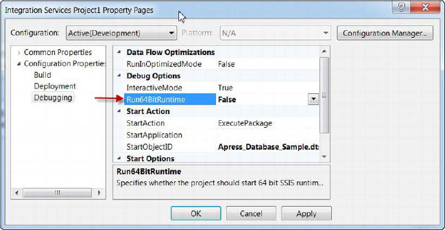
Figure 7-30. Setting the SSIS project to run in 32-bit mode
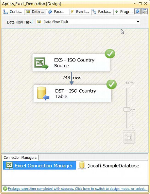
Figure 7-31. Successful run of Excel spreadsheet import to SQL Server table
Whereas the Excel source adapter lets you pull data from Excel spreadsheets into your data flow, the Excel destination allows you to output data from a data flow to an Excel spreadsheet. To demonstrate, we’ll pull the contents of the Country table we just populated from the database and output it to a new spreadsheet.
We’ll add a new Excel Connection Manager to the SSIS package and point it at a new, mostly empty spreadsheet. The new spreadsheet will have only the names of the columns in the first row, as shown in Figure 7-32.

Figure 7-32. New SSIS destination workbook, empty except for column headings
Next we’ll add an OLE DB source adapter and an Excel destination adapter to an empty data flow. After we configure the OLE DB source to pull data from the Country table in the database, we link the OLE DB source output to the Excel destination input. The final step is to configure the Excel destination. In the Excel Destination Editor, we selected the newly created Excel Connection Manager, set the data access mode to Table or View, and chose the name of the first worksheet, Sheet1$, as shown in Figure 7-33.

Figure 7-33. Configuring the Excel destination adapter in the Excel Destination Editor
Raw Files
Whenever you read from or write to a flat file, there are thousands of data conversions taking place in the background. Consider an integer number such as 2,147,483,647. This number uses only 4 bytes of memory in your computer. But when you write it out to a flat file, it’s converted to a string of numeric digits 10 characters long. That’s more than double the storage and a performance hit because of the conversion. When you read the number back in from a flat file, you have to read in 10 characters and you get hit with another conversion penalty. Granted, the size difference and performance impact isn’t that much for a single number, but multiply that by 10 columns and 1,000,000 rows (which is not an unreasonable example), and suddenly you’re talking about a noticeable change in both performance and storage space.
For day-to-day file transfers and imports/exports from and to other systems, flat files are the way to go. In a lot of cases, flat files aren’t all that large, so the size and performance differences aren’t significant. But more important, when transferring data between systems, you can’t go wrong with plain text. Accounting for some variation between character sets, every system reads text, and every system writes text.
Sometimes, however, you may find a need to temporarily store large volumes of partially processed data during processing. A common example is when a large number of rows have been pushed through an SSIS package, a lot of processing has taken place, and you need to pick up the data in another SSIS package (or a different data flow in the same package) for further processing. To maximize efficiency of your SSIS interpackage processing, raw files are hard to beat.
Raw files are specialized binary format files that eliminate a lot of the conversion overhead associated with normal flat files. Raw files store your data in binary format, so that those 4-byte integers are stored in exactly 4 bytes. Raw files also store metadata about your columns, so the binary data in the raw file can’t be accidentally read in as the wrong format. The Raw File destination adapter lets you output data from your data flow to a raw file; the Raw File source adapter lets you read a raw file back into your data flow. The raw file provides an efficient intermediate format for serializing temporary results.
Just as one example of the use of raw files, we recently ran into a situation where we had to dump a large amount of data from a Microsoft Access database using 32-bit Jet 4.0 drivers and import the data into a SQL Server database using 64-bit drivers. You can’t mix 32-bit and 64-bit drivers in the same package, so the solution was to create two packages: one to extract the data from Access into a raw file and one to import the data into SQL Server. We ran the Access extract package using the SSIS 32-bit runtime and the SQL Server import package using the SSIS 64-bit runtime. This is just one example, but there are plenty more in which the raw file produces efficient temporary storage of your intermediate results. Anytime you need to temporarily store partially processed data, consider raw files.
XML Files
The XML source adapter lets you use an XML file with an XML Schema document (XSD) as a source for your data flow. The XML Source uses the XSD you provide to extract the data values from your XML file and output it in columns. If you don’t have an XSD file, this component will generate a simple one for you. The XML source adapter is useful for relatively simple XML files, or for extracting well-defined subsets of data from more-complex XML files.
![]() NOTE: We recommend the book SSIS Design Patterns by Matt Masson , Tim Mitchell , Jessica Moss , Michelle Ufford , Andy Leonard (Apress, 2012), which devotes an entire chapter to loading XML files with SSIS.
NOTE: We recommend the book SSIS Design Patterns by Matt Masson , Tim Mitchell , Jessica Moss , Michelle Ufford , Andy Leonard (Apress, 2012), which devotes an entire chapter to loading XML files with SSIS.
Special-Purpose Adapters
SSIS has two special-purpose destination adapters, which provide additional functionality, such as writing to in-memory recordsets or to SQL Server Analysis Services (SSAS). These adapters are as follows:
Recordset: The SSIS Recordset destination adapter lets you populate an in-memory recordset. One of the most common uses of the in-memory recordset is to populate it via the data flow and later iterate it with a Foreach Loop Container.
DataReader: The DataReader destination adapter outputs data in a format compatible with the .NET DataReader interface, which can be picked up and consumed by an application that can read a DataReader. SQL Server Reporting Services (SSRS) reports, for instance, can be set to consume the output of an SSIS package using the DataReader interface.
Analysis Services
In addition to all the source and destination adapters we’ve covered in this chapter, SSIS provides destination adapters for SQL Server Analysis Services (SSAS). This section provides an overview of SSAS capabilities, and Chapter 14 presents detailed information about SSIS’s Analysis Services functionality. Table 7-5 lists SSIS’s Analysis Services destinations.

Summary
In this chapter, we discussed SSIS’s source and destination adapters, the key components required to move data into and out of your SSIS data flows. We began this chapter with a discussion of SSIS’s Source and Destination Assistants, two new features designed to make creating source and destination adapters a little more convenient. We then detailed how to create and use different flavors of database-specific source and destination adapters, which are among the most commonly used types of data flow adapters.
Next we discussed the various types of files that SSIS supports reading from and writing to, including flat files, Excel spreadsheets, raw files, and XML. We also talked about the special-purpose destinations: the Recordset and DataReader destination adapters, and we finished up with an introduction to the Analysis Services destinations—a conversation we will pick up again in Chapter 14.
In the next chapter , we introduce the third type of data flow components—transformations.