C H A P T E R  3

Hello World—Your First SSIS 2012 Package

Take the first step in faith. You don't have to see the whole staircase, just take the first step.

—Civil Rights Movement leader Martin Luther King Jr.

In the previous chapter, we introduced you to SQL Server 11’s development tools, BIDS and SSMS. Before we start discussing the in-depth details, we will walk you through some example packages to demonstrate the capabilities of this powerful toolset. As a developer, it is much easier for you to gain an understanding after you’ve tried out the tools for yourself. This chapter teaches you how to start with the simplest package, consisting of a Data Flow task that will have only a source and a destination. After walking you through creating the easy package, we will guide you through a more complex, real-life example of a package. This package’s goal will be to emulate some of the potential requirements that may become a part of your ETL process, and as such is a relatively complex example to be introduced in the third chapter.

The reason we are not covering all the details before we lead you to the first package is that SSIS has a vast set of tools, a majority of which will not be used together at the same time. Most projects will utilize only a few of the connection managers, for example, while SSIS has a much larger number available. Depending on the requirements of the project, the processes handled by SSIS might have to be divided with other tools. This chapter provides a quick glance at some of the capabilities of SSIS.

For this chapter, we took our data from the US Census Bureau web site, http://2010.census.gov/2010census/data/. We use the Apportionment and Population Density datasets in this chapter. The only change we made to this data is to remove some header and footer records to keep the introduction to developing SSIS 11 packages simple. The actual data itself was not modified. Apportionment refers to the dividing of the total seats in the House of the Representatives among the 50 states, depending on their population. Population Density reports the average population per square mile of the state.

Integration Services Project

As we discussed in the previous chapter, the key to SSIS development is the Integration Services pin BIDS. The project file can organize all the files that are related to an ETL process. When you first create a project, Visual Studio will automatically create the first package for the project and name it Package.dtsx. The first package will be completely empty, and the initial designer will show the control flow. You have the ability to rename the package as soon as it is generated.

Key Package Properties

The package has properties that are organized according to the function they provide. These properties carry out the functional and nonfunctional requirements of the ETL process. Functional requirements comprise the principles of extract, transform, and load (ETL), whereas nonfunctional requirements take care of the robustness, performance and efficiency, maintainability, security, scalability, reliability, and overall quality of the ETL process. There are a few properties that we recommend you look over when creating new packages in the project:

Name can be modified through Visual Studio’s Solution Explorer. The benefits of modifying through Visual Studio’s Solution Explorer as opposed to modifying through the file system or the property field in the package include the automatic recognition by the project file and the automatic renaming of the package name property. Upon creation, this value is defaulted to the name assigned by Visual Studio.

DelayValidation determines whether the package objects will validate when the package is opened for editing. By default, this property is set to False, meaning that all the objects will validate when the package is opened. By setting this property to False, you will validate only during runtime. This can be dangerous to do during the development phase if there are Data Definition Language, DDL, changes or structural changes to either the sources or the destinations. It may be useful when developing large packages, by allowing the packages to open/load faster, but we recommend keeping the SSIS packages as modular as possible. We discuss the different options for modularity in Section 2 of this book.

ID provides a unique identifier for the package. This property becomes important when considering logging options. This ID will distinguish the packages that are run for a particular execution. A new identifier is generated when a new package is added to the project, but when an existing package is added or a package is copied and pasted in Solution Explorer, the identifier of the original package is carried over. This value is not directly modifiable, but there is an option to generate a new ID.

ProtectionLevel manages the sensitive data stored in the package. By default, this property is set to EncryptSensitiveWithUserKey. This option encrypts the whole package with a key that will identify it with the current user. Only the current user will be able to load the package with all the information. Other users will see only blanks for usernames, passwords, and other sensitive data. We recommend using the DontSaveSensitive option, especially if multiple developers will be working on the same set of packages. Sensitive data can be stored in configuration files. We discuss the security aspects of developing and deploying packages in Chapter 19.

Package Annotations

After taking a look at the properties set on the new package, one of the first things we recommend is adding an annotation to the package. This can be done by right-clicking on the background of the current designer view and selecting Add Annotation. Annotations can be used to document the package so that fellow developers can easily identify the purpose of the package without having to open and read through all the tasks. Thoroughly examining the packages can be saved for debugging time. The kind of information the annotations should contain is identified in Figure 3-1.

Figure 3-1. Recommended annotation to control flow

The name represents the name of the current package. This is displayed in several places in Visual Studio, but with the vast improvements to the XML behind the SSIS packages, don’t be surprised if you have to look there for certain information. The annotation string itself is stored in the CDATA at the bottom of the package XML.

The modified date simply dates the last set of changes made to the package. This piece will help in the absence of a code repository. The file system modified date is not always accurate in capturing actual changes to SSIS packages. Clicking the OK button on many of the designers as well as moving objects around in the designer tabs will cause Visual Studio to recognize changes even if there aren’t any functional changes. This can cause the file system to inaccurately represent functional changes to the packages.

The purpose simply identifies the objectives of the package. Modular programming is characterized by having separate, interchangeable code blocks or modules. We cover some design patterns that will enable you to maintain this practice with SSIS 11 in Section 2 of this book. The purpose covers the end state after the execution of the package—which data elements have been moved, which items have been moved around on the file system, the execution of stored procedures, and so forth. This is meant to be a high-level description rather than a detailed description but essentially will depend on your design of the ETL process.

Parameters and variables are related in that they can be used to pass values between packages. Parameters are external values that can be set prior to the execution of the package. Variables are internal mechanisms to pass information between packages. In prior versions of SQL Server Integration Services, variables served both purposes through configurations either by using configuration files to assign values or by inheriting values through parent variables. It is important to identify parameters because they are accessible to all the packages in a project; this construct becomes extremely useful when utilizing the parent-child package design. The parent package can automatically detect the parameters defined in the child package as well as assign which variables or parameters to pass along to it.

Variables can now be used for the sole purpose of passing values among packages without modification from external processes. When assigning parameters and variables, they are available in the same drop-down list along with the system variables. You also have the option to write expressions to assign parameter values to variables. Variables are passed to a child package by reference rather than by value. Any modification made to the value will require a Script task in the child package to propagate the change back up to the parent package. There is an alternative to using the Script task to modify the parent package, which allows you to directly access the variable. However, this method also causes the executables accessing the variables within the child package to error during the runtime, when the child package is executed on its own. We discuss these options in Chapter 16.

Variable listing is sensitive to the scope of the variables. The scope of a variable can be from the package as a whole or within a specific container, task, or event handler. With multiple variables, you can easily lose track of them all, so the annotation can save a lot of digging around. The Package Explorer tab and the Show Variables of All Scopes option in the Parameters and Variables toolbar allow the same functionality, but with the annotation, you can document the role they play in the process.

Package Property Categories

The package properties are divided into categories to group them by the function they provide. These categories are generally broad and contain a lot more configurable properties than the main ones outlined in the preceding section. These categories and their properties address some of the nonfunctional capabilities of SSIS 11. We briefly introduce the categories here and provide more in-depth analysis in the later chapters:

Checkpoint properties control the restart ability of SSIS package execution. You have to define a file path and name for the progress to be stored during execution. In the event of a failure, this file will be used to restart the process at the task at which it previously failed. This functionality by itself will not handle the rollback of committed data. After a successful execution, this file is automatically deleted.

Execution properties define the runtime aspects of the package. These include the number of failures that the package can tolerate and how to treat the failures of nested containers with respect to the success of the parent container. Performance tuning can also start with the properties in this section. If memory overflows become an issue, the number of concurrent executables can be limited.

Identification properties are used to uniquely recognize packages. These properties include some of the ones listed previously (specifically, Name and ID). Other information that the package can capture is the machine that it was created on and the user who created it. Another important property that is categorized here is Description, which is free-form text.

Misc properties are a mixture of those that cannot be cleanly classified in the other categories. This category includes disparate properties that vary in function from logging behavior of the package execution to listing configurations created for the package.

Security properties handle the sensitive information that may be stored in a package. The main property in this segment, ProtectionLevel, was listed earlier. These properties can be configured depending on the different environments used for development, testing, and production. Some settings will allow you to move the packages between environments without causing authentication issues.

Hello World

With a brief introduction to SSIS 11 package properties under your belt, let us dive right into creating a package. The first step in developing a package in Visual Studio requires a project. For this particular chapter, we created a project aptly titled Chap3_HelloWorld. Figure 3-2 demonstrates how to create a new Integration Services project within Visual Studio. You access the dialog box by going to the File menu on the toolbar and choosing New ä Project. An alternative to this is to use the Recent Projects pane on the Start page. There is hyperlink to create a Project at the bottom.

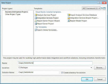
Figure 3-2. Creating a new Integration Services project

Following are some of the elements within the dialog box, and a brief description of their purpose:

• The Name text field in the dialog box assigns the name to the project file. This name should be sufficiently broad to cover the various packages that will be stored. Because we are trying to demonstrate only a simple package, the project name refers to a simple process.
• The Location field indicates the directory where the project will be stored on the file system during development. For simplicity, we created a short folder path to store our packages.
• The Solution Name field is automatically populated with the same value as is provided in the Name field, but it can be changed if the name does not suit the solution.
• The Create Directory for Solution check box is extremely useful for keeping the projects organized. It will create a subfolder within the defined Location and place all the files (.database, .dtproj, .dtproj.user, .dtsx, and so forth) and subfolders required for building and deploying within it.

After the project is created, Visual Studio will automatically generate a package and name it Package.dtsx. One of the first steps we recommend that you perform is to modify this name to a more appropriate and descriptive name. If you change it directly through Solution Explorer, you will get a dialog box asking you to confirm a change to the Name property of the package. If you change the name of the package through the Properties window, you will not get a dialog box to confirm a change to the file name. This behavior allows the two to be out of sync, but there is no reason to have such a scenario. We recommend that you keep them in sync.

Because we are not creating a complex package with large amounts of metadata, we are going to leave the DelayValidation property to False. This package will simply take data from a flat file and move it to a SQL Server 11 database without any transformations. This is the simplest ETL task SSIS can perform, taking data from a source storage platform and placing it in a destination storage platform. We will also skip over the ID generation because we did not copy this package from an existing one.

We will set ProtectionLevel to DontSaveSensitive. This will allow us to work on the package without having to remember a password or having to use the same machine through a common user account. It will also force us to store any required connection information in a different file other than the package. We encourage you to store sensitive information in configuration files for both the security of storing the information only once and the ability to limit access to this file.

After all the desired properties are set, we can start the actual development of the package. We recommend that you add an annotation like the one shown in Figure 3-1 that outlines the basic design we are going to implement for the ETL process. With the annotation in place, we know the function of all the objects in the package. The first step toward the ETL process is identifying the data you want to extract, the location of the data, and some rudimentary data (metadata) about the data. When handling flat files, metadata becomes crucial because a low estimation of column lengths will result in truncation.

Flat File Source Connection

The first object we will add to the package is a flat file connection. We do this by right-clicking in the Connection Managers pane at the bottom of the designer and selecting New Flat File Connection. This opens the Flat File Connection Manager Editor, depicted in Figure 3-3. We recommend that you replace the default name of the connection with one that will enable you to easily identify the data to which the manager is providing access. The name of the connection must be unique. In addition, we also recommend writing a short description of the manager in the Description field. These two fields will reappear in all of the pages listed in the left panel of the editor.

Figure 3-3. Flat File Connection Manager Editor —General properties

The File Name field stores the folder path and the file name that will be associated with this particular data set. The Browse button allows you to use Windows Explorer to locate the file and automatically populate the path into the field. When using the Browse option, it is important to note that the default file type selected is .txt. In our case, we are using a .csv file for our data, so we had to change the file type to be able to view it in Windows Explorer. The Locale drop-down provides a list of regions for language-specific ordering of time formats. The Unicode check box defines the dataset to use Unicode and will disable the Code Page ability. The Code Page option enables you to define non-Unicode code pages for the flat file.

The Format section of the Flat File Connection Manager Editor’s General page allows you to define how SSIS will read in the file. There are three formats to choose from: Delimited, Fixed Width, and Ragged Right. Delimited, the default format, enables you to define the delimiter in the Columns tab. For .csv (comma-separated values) files, the delimiter is a comma. Fixed Width defines the columns in the flat file as having a determined column length for each of the columns. The length is measured in characters. A ruler helps you define the individual characters for each column. You can choose from various fonts in order to accurately display the characters. Ragged Right follows the same rules as Fixed Width except for the last column. The last column has a row delimiter rather than a fixed width.

The Text Qualifier text box allows you to specify the qualifiers that denote text data. The most common way to qualify text is by using quotes. The Header Row Delimiter list defines the characters that mark the first row of data. Usually, this is the same as the row delimiter. For .csv files, the row delimiter is a carriage return immediately followed by a line feed. When we downloaded the data from the Census Bureau’s web site, we cleaned up some of the header records so that only the column names and the actual data remained. The check box labeled Column Names in the First Data Row allows SSIS to easily read in the file and capture the column names defined in the .csv file, as demonstrated by Figure 3-4. This cleans up the names so that you don’t see names such as Column1, Column2, and so forth. and replaces those generic names with the actual column headers defined in the .csv file.

Figure 3-4. Flat File Connection Manager Editor—Columns page

The Columns page of the Flat File Connection Manager Editor allows you to define the row delimiter and the column delimiter. With .csv files, the rows are delimited with carriage returns and line feeds, and the columns are delimited with commas. After setting these values, you can preview a sample of the rows using the delimiter values defined. If you need to make any changes to the delimiter, you can refresh the Preview pane to see how the changes will impact the connection manager’s reading of the file. The Reset Columns button will remove all the columns except the original columns.

With the Fixed Width option, the Preview pane has a ruler at the top. In this mode, the preview will ignore the new line characters in the actual file. The marks along the ruler will demarcate the columns’ widths. Each column can have its width defined using the ruler. The Preview pane will visually assist with how the connection manager will read in the data. The Ragged Right option will have an extra field that will allow you to define the row delimiters.

The Advanced page of the Flat File Connection Manager Editor, shown in Figure 3-5, allows you to modify the metadata of each column. The columns represented here are dependent on the columns defined through the Columns page. In the Advanced page, you can modify each of the columns’ names, column delimiter, data type, output column width, and text qualified. For the last column in the flat file, the column delimiter will be the row delimiter. Depending on the data type chosen (numeric data), data precision and data scale become available. The column type determines these options, and for the delimited formats these are the columns available. For the other two formats, you can define the input column widths individually. Changes here will be reflected in the Preview pane on the Columns page.

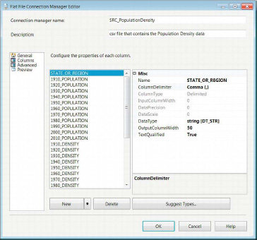
Figure 3-5. Flat File Connection Manager Editor—Advanced page

The Preview page displays a sample dataset from the source according to the metadata defined in the other pages. Figure 3-6 demonstrates this page of the Flat File Connection Manager Editor. It also has the option to skip data rows in the source. This is a different option than the one on the General page. The General page option allows header rows to be ignored so that the appropriate row can be used as the source for the column names. This Preview page option will ignore rows that immediately follow the row containing the column headers.

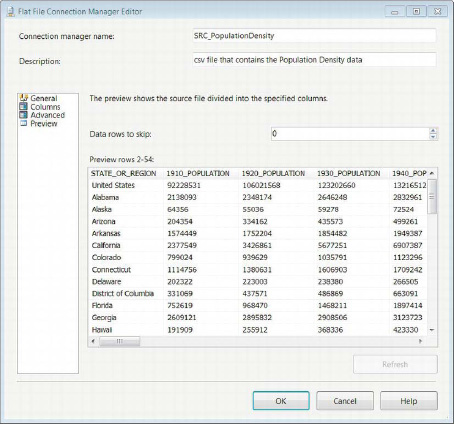
Figure 3-6. Flat File Connection Manager Editor—Preview page

OLE DB Destination Connection

With the source of our data ready for extraction, we need to set up the destination for loading. For this example, we will be using a SQL Server 11 database as the destination. We will create a table that will fit the metadata of the source, essentially taking the data from a file system flat file and storing it in a relational database management system (RDBMS). The first step in creating an Object Linking and Embedding Database, OLE DB, Connection Manager is to right-click in the Connection Managers pane in the designer window. Here you will have to add a data connection to a server, using the dialog box shown in Figure 3-7, if you do not already have one. You will need the login information ready when you are creating the data connection. If you do not have the server name, you can put in the IP address of the server, or if you want to load the data in a local instance on your machine, you can call it by using the (local)instance name.

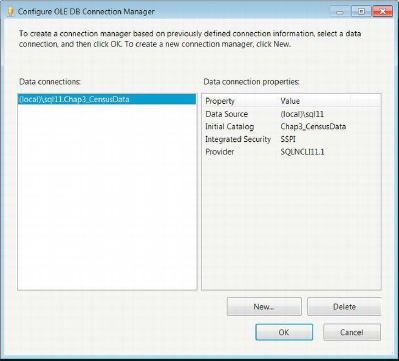
Figure 3-7. Configuring the OLE DB Connection Manager

This manager allows you to store data connections that you use in SSIS. This is not limited to connections used within a particular project. You can configure the new connections by using the wizard shown in Figure 3-8. By default, the connections stored within the connection manager will have names in the following format: DataSource.InitialCatalog. The Data Connection Properties pane will show the connection string information and the default values for that particular connection. Clicking the New button will prompt the Connection Manager Wizard depicted in Figure 3-8. Connection managers are not limited to extract or load duties; they can perform both tasks, although doing both simultaneously may risk contention issues.

The Data Connection Properties pane shows all the information needed to extract—or in our case, load—data into a SQL Server 11 database. The Data Source refers to the server and the name of the instance on the RDBMS on the server. The IP address can be just as easily used, but we recommend using the name of the machine wherever possible. The Initial Catalog is the database in which the data will be extracted from or loaded to. The Integrated Security property determines how the database is accessed: whether a username and password are used or Windows Authentication passes on the credentials. For our example, we will be using Windows Authentication. The Provider is the driver that is used to connect to the database. SQLNCLI1.1 is the driver required to connect to a SQL Server 11 database.

Figure 3-8. Connection Manager—Connection page

On the Connection page, you are asked to provide all the details needed to connect to a particular database. In this case, we want the database in which we will be storing the Population Density data. This information can be easily referenced in the Data Connection Properties pane on the Configure OLE DB Connection Manager wizard after the connection has been created. The wizard allows you to easily review all the previously created connections for reusability. The Server Name of the connection manager must also include the instance name. The radio buttons below that field indicate the access mode to use. When using Windows Authentication, make sure you have the proper credentials to access the server and database. Without access, you will not be able to gather or validate the required metadata. For each connection, you have to specify the database you intend to use. Utilizing configuration files will allow you to store the connection information in a separate file. This allows changes to propagate across multiple packages that are configured to use the file rather than manually opening and updating each instance of the connection manager. The Test Connection button uses the information provided to ping the server and database. It is a quick way to test your credentials and validate access to the selected database. The All page of the Connection Manager dialog box, shown in Figure 3-9, gives you access to all the available properties of the connection.

Figure 3-9. Connection Manager—All page

Utilizing the All page provides properties beyond those in the Connection page. This page allows you to fully modify the connection manager to meet your needs. You can define connection timeouts to provide a maximum limit in how long a query can run. We would not recommend tweaking these properties unless you need to for very specific reasons. By default, these settings should provide the optimal performance that you require. After you add the connection manager, we recommend that you rename it immediately so that when you try to access it later, you can easily identify it.

Data Flow Task

After adding the connection managers for the source and destinations of our dataset, we can move on to adding the executable that will extract and load the Population Density data. The Data Flow task can be found in the Favorites subsection of the SSIS Toolbox. It is here by default and can be moved around if you do not use it too often. Figure 3-10 illustrates the control flow pane with a single Data Flow Task.

Figure 3-10. HelloWorld.dtsx—control flow

Using the naming convention introduced by Jamie Thomson, we named the preceding executable DFT_MovePopulationDensityData. The DFT indicates that it is a Data Flow task. The rest of the name describes the function of the Data Flow task. Each of the control flow components has its own symbol, allowing you to readily recognize the object. The data flow symbol has two cylinders with an arrow from one pointing to the other.

You can add the connection managers in a different order than we have done in this package. We approached creating this package from a step-by-step manner in which identifying the source and destinations was the first agenda. As you will see in the sections with the assistants, you can add connection managers as you are adding the components to Data Flow. We see this as providing a chance to create ad hoc managers rather than creating the sources and destinations through a planned process.

Source Component

With the connection manager in place for the Population Density file and the Data Flow task to extract the data, we can add the source component that will open the connection and read in the data. In SSIS 11, the addition of the Source Assistant greatly helps organize the different connection managers we created. Figure 3-11 demonstrates how the Source Assistant enables you to quickly add a source component for your desired connection. In this example, the source we are looking for is SRC_PopulationDensity. If you choose to, you can add a new connection manager here for your source data by selecting <New> and clicking the OK button.

Figure 3-11. Source Assistant

The Types pane contains all the connection managers that are currently supported by your machine. Drivers for other connection managers such as DB2 can be downloaded from Microsoft’s web site. For our package, we are concerned with only the Flat File source, and in the Connection Managers pane, all the managers of that type are listed. In this package, HelloWorld.dtsx, there is only one such manager. The bottom pane shows the connection information for this particular flat file, so you can even see the file name and path. In previous versions of SSIS, you had to know the connection information for each manager before you added the source component. The Source Assistant did not exist to show you the connection string for the different managers. The naming convention used for the connection managers is important in this regard. After clicking the OK button, you will automatically add the component to DFT_MovePopulationDensityData. By default, the name of the component is Flat File Source, but by using the defined naming conventions, we changed the name to FF_SRC_PopulationDensity. The component automatically resizes when you type in the name so that you get a clear idea of how much space the component will use up in the window.

Destination Component

With our source component in place, we can now add the destination for our data. The other new assistant that has been added to SSIS 11 is the Destination Assistant. This assistant offers the same organizational help that the Source Assistant provides. One of the key features of the assistant is the connection information that is displayed in the bottom of the pane, as depicted in Figure 3-12. The option to add a new connection manager is available through the assistant. Naming the connection managers appropriately will make identifying the proper connection much easier.

Figure 3-12. Destination Assistant

After we select the connection manager we want, DES_Chap3_CensusData, we can add it to the data flow by clicking the OK button. The component will be added with the default name of OLE DB Destination. We will adhere to the naming convention and rename it OLE_DST_CensusData. Just as was the case with the source component, it will automatically resize to fit the name provided.

Data Flow Path

After we have both the source and the destination components in the Data Flow task, we need to instruct SSIS to move the data from the source to the destination. This is done by defining a path for the data flow. To add the path, you have to click the source component. You will see two arrows appear at the bottom of the component. The green arrow represents the flow of data after a successful read, and the red redirects rows that fail during the read. The green arrow is recognized by SSIS as the Flat File Source output, and the red arrow is referred to as the Flat File Source Error Output. These two arrows are shown in Figure 3-13.

Figure 3-13. Source component—outputs

The data flow path can simply be created by clicking and dragging the green arrow from the source component to the destination component. The other option is to use the wizard to Add Path in the Data Flow. This wizard can be accessed by right-clicking the source component and selecting Add Path. This opens a dialog box enabling you to choose the components and the direction of the path, as shown in Figure 3-14.

Figure 3-14. Data FlowCreate New Connector

With this connector wizard, we can define the direction of the data flow. This connector wizard will affect the settings of the wizard that appears after this one, as depicted in Figure 3-15.

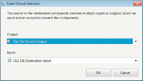
Figure 3-15. Input Output Selection

This wizard allows you to match the inputs and the outputs of the source and destination components. For the output, you have two options: the Flat File Source Output and the Flat File Source Error Output. Because we want the actual data from the file, we selected the Flat File Source Output. The OLE DB destination component can accept only one input. After you click OK, the data path will be created between these two components using the outputs and inputs that were defined. But creating the data path is not the final step; we need to map the columns between the source and the destination.

Mapping

As you recall, we had to define all the columns that we were expecting from the source. The same process is required when moving the data to a destination. After we create the data path between the source and the destination, Visual Studio provides a small reminder of this fact through a small red x on the destination component, as can be seen in Figure 3-16. The error will propagate to the control-flow-level executable, so you will see the x on DFT_MovePopulationDensityData as well.

Figure 3-16. Data Flow task—mapping error OLE DB destination

You can identify the reason behind the errors by holding your cursor on top of the x mark. In our case, we did not define the destination table for our data. To fix this issue, we have to double-click the destination component to open the OLE DB Destination Editor. The editor, shown in Figure 3-17, allows you to modify the connection manager to be used as well as some options regarding the actual insertion of data into the database.

Figure 3-17. Fixing the error by using the OLE DB Destination Editor

The OLE DB Connection Manager drop-down list allows you to change the connection manager from the one selected when the Destination Assistant was used. The Data Access Mode list provides you with a few options on how to load the data. The Table or View option loads data into a table or view defined in the destination database. This option fires insert statements for each individual row. For small datasets, these transactions may seem fast, but as soon as the data volumes start increasing, you will experience a bottleneck using this option. The Table or View – Fast Load option is optimized for bulk inserts. This option is the default when setting up the destination component. The Table Name or View Name Variable option uses a variable whose value is the name of the destination table. This option also uses only row-by-row insert statements to load the data. Table Name or View Name Variable – Fast Load also utilizes the value of a variable to determine the destination table but it is optimized for bulk insert. The SQL Command option utilizes a SQL query to load the data. This query will execute for each record that appears in the input of the destination component.

We do not have a table ready to load the data from the source, but the OLE DB Destination Editor has the ability to generate a CREATE TABLE script based on the metadata passed to its input. The table script it generates for this particular dataset is shown in Listing 3-1. If we had removed columns from the pipeline prior to passing them to the destination component, they would not have been added to this create script. The bold code denotes the changes we made to the script to conform to our naming standards. By default, the table name was OLE_DST_CensusData, the name given to the component. The editor does not specify table schema when it generates the create table script. If the table you want to load the data into is already created, it is available in the drop-down list.

The column names and lengths were defined based on the metadata defined in the Flat File Connection Manager. Because we did not define the columns as Unicode, the default data types for all the columns are varchar. This create script is made available through an editable text box that opens when you click the New button for the destination table selection. With the script modified to meet our needs, we need to execute it on the destination database to create the table.

After we create the table on the database, it will appear in the drop-down list of destination tables. Because the column names and data types match exactly for the columns in the destination input, the mapping is automatically created by SSIS, as shown in Figure 3-18. In order to see the mapping, you need to click the Mappings option in the left pane of the editor.

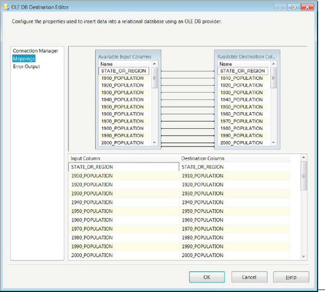
Figure 3-18. OLE DB Destination EditorMappings page

To create mappings from the input columns to the destination, you have two options. You can use the UI on the top half of the editor, which allows you to click and drag the input column to its matching destination column. Alternatively, you can use the bottom half of the screen, where the input columns are shown in drop-down lists next to each destination column. You can map an input column to only one destination column. If you want to map the same column to multiple destinations, you will have to use a component in the pipeline that will add the duplicate column.

Before we run this package in Visual Studio, we have to make sure that the project ProtectionLevel property matches the value set in the package, DontSaveSensitive. Without changing this property, Visual Studio will report build errors and will not allow us to execute the package. After all the components have been created and the properties set, we can take a quick look at the Package Explorer window to quickly review the objects in the package. The Package Explorer for HelloWorld.dtsx is shown in Figure 3-19.

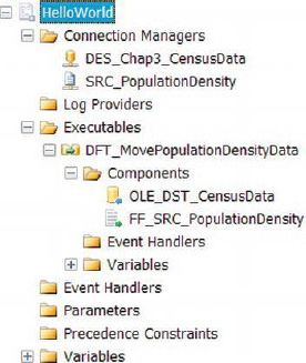
Figure 3-19. HelloWorld.dtsx—Package Explorer

The Variables folder in Figure 3-19 is expandable because there are default system variables that are created for all the packages. They are created with Package scope, so all defined executables and containers will have access to them. Because this package is designed to be as simple as possible, a majority of the objects have been skipped. We have only one executable, DFT_MovePopulationDensityData, on the control flow so we do not see any precedence constraints.

Aside from offering an organized view of the package’s object, the Package Explorer design window also allows you to quickly navigate to the object that requires modification. Double-clicking the individual connection manager will open its editor. Double-clicking the Data Flow task will open that particular Data Flow task’s design window.

Execution

We have finally arrived at the fruits of our labor. We have set up the package, and all the objects are in place to allow us to move data from the flat file to the SQL Server 11 database. Using Visual Studio to execute the package requires opening the package as a part of a project. Visual Studio performs build operations before each debugging operation by default. This allows you to see the progress of each component and executable. Figure 3-20 displays the Standard toolbar with the Start Debugging button highlighted. Another option to execute a package in Visual Studio is to right-click the package and select Execute Package. The solution file also starts the debug mode; to use this method, you have to right-click the solution name in Solution Explorer, going to the Debug Group and then selecting Start New Instance.

Figure 3-20. Visual Studio Standard toolbar

There are three colors associated with the Visual Studio debug mode for SSIS 11: green denoting success, yellow denoting in progress, and red denoting failure. Figure 3-21 shows the output of the debug operation of this package. Visual Studio provides a row count for each data path; for this simple package, there is only one. This output informs us that 53 rows were extracted from the flat file and successfully inserted into the destination table.

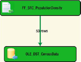
Figure 3-21. DFT_MovePopulationDensityData—execution visuals

Another option to execute the package is to use the Start Without Debugging option in the Debug menu on the menu bar. This will prompt Visual Studio to call dtexec.exe and provide it with the proper parameters to execute the package. One downside to this option is that Visual Studio does not provide the parameter that limits reporting to errors only. Executing the package without a limit on reporting will result in a massive output that will most likely overrun the screen buffer for the command prompt. We recommend using the command prompt to call dtexec.exe yourself with the proper parameters you desire. You can even store the output to a file to review the execution details. We cover this option fully in Chapter 26.

To validate that the data has been loaded into the database, you can run queries to test the ETL process results. Listing 3-2 shows a quick way to verify that the data loaded properly. The first query performs a row count to show the number of records in the table. The second query will output all the records that are stored in the table.

By querying the data, you are inadvertently enjoying one of the benefits of having data in an RDBMS as opposed to a flat file. This particular dataset uses the column name to delineate the data that it contains. This is a relatively denormalized dataset forcing you to select a particular year and statistic combination to view the data. In 2020, the only way to update this data would be to add new columns to support the new data. With data normalization, we tend to prefer loading data rather than modifying existing table structures. For a more complex and real-world example, the next package will illustrate how we might go about normalizing the data on the fly by using SSIS 11.

Real World

The simple package example quickly exposed you to SSIS 11 development. However, in everyday situations, the requirements will not be as simple. This next example shows you some functional requirements you might face in the workplace. In this package, we will combine the Population Density data with the Apportionment data and store it as a query-friendly dataset in the database. To do this, we will build on the work we did for the Hello World example.

In order to leverage the development on HelloWorld.dtsx, we simply added the package to a new solution, Chap3_RealWorld. After we created the new solution, we deleted the default Package.dtsx and then right-clicked the solution file and selected Add Existing Package in the Add Group. After it was added, we renamed it in Visual Studio to RealWorld.dtsx. Adding it to the new project simply creates a copy of the file. If you create all your solutions in one folder, you will create a copy named RealWorld (1).dtsx. Figure 3-22 shows the executables that we created to allow the package multiple runs without having to externally delete previous data.

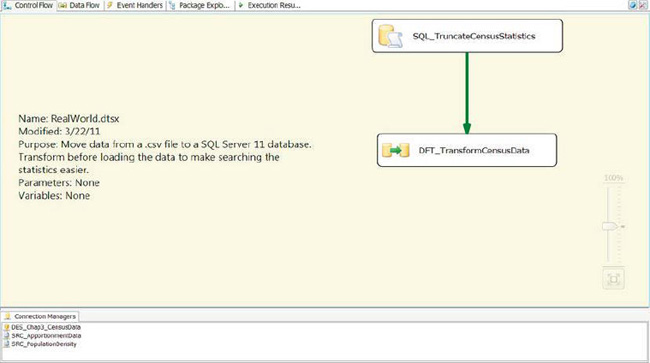
Figure 3-22. RealWorld package added to new Chap3_RealWorld solution

Control Flow

In addition to the two connection managers we had for the first package, we added a third connection manager, SRC_ApportionmentData, so that we may be able to extract the Apportionment dataset. We also added an Execute SQL task executable, SQL_TruncateCensusStatistics, in order to run the package without having to truncate the table between executions of the package. The Data Flow task, DFT_TransformCensusData, is more complex in comparison to DFT_MovePopulationDensityData because of the components we had to use to meet the requirements. The transformation components we will introduce to you are the Derived Column, Sort, Merge Join, and Unpivot components.

Execute SQL Task

SQL_TruncateCensusStatistics requires an OLE DB connection for it to execute the SQL statement contained within it. This executable can be used for many purposes, from extracting data from a database and storing it as an object for the SSIS package to access to executing update statements. For our purposes, we will use it to truncate the table every time we run the package. The green arrow, a precedence constraint, ensures that the Execute SQL task completes execution before the Data Flow task starts executing. DFT_TransformCensusData will execute only on the successful completion of SQL_TruncateCensusStatistics. Figure 3-22 shows the configuration of the Execute SQL task. There are some key attributes of the task that we modified before we placed the executable:

Name is a unique identifier for the task in the control flow. No two tasks of the same type can have the same name. This name is the label that is displayed in the control flow designer.

Description is a text field that provides a short explanation of the task’s function in the package. It is not required to modify this attribute but it can help those who are new to the package understand the process more easily.

Connection, a required attribute, is blank by default. Because we want to truncate the destination table, we use the same connection manager as the OLE DB destination component. There is no need to create a new connection manager just for the Execute SQL task.

SQL Statement contains the DDL, Data Manipulation Language( DML), or Data Access Language, DAL, statements that need to be executed. As you can see in Figure 3-23, we put in one statement followed by a batch terminator and GO. When you modify the statement, a text editor opens and you can type the statement. Without the text editor, you cannot place GO on a new line and thus will have an error when you execute the package.

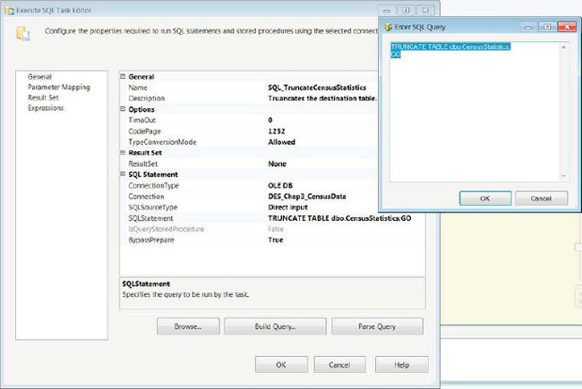
Figure 3-23. SQL_TruncateCensusStatistics—configuration

Data Flow Task

The Data Flow task executable is the workhorse of RealWorld.dtsx. It extracts data from the flat files, joins the data in the two files, and outputs the data in a normalized format. This process can be done by pulling the data directly into SQL Server in a staging table and then using SQL to convert the data into the desired form. Strictly in terms of I/O, this second approach is usually inefficient because it requires two passes of the data. The first read extracts it from the flat file source, and the second one extracts it from the staging table. The process we implemented takes one pass of the file, and because SSIS is optimized for row-by-row operations, it does add extra overhead to transform the data on the fly. The only risk in this method is the use of the Sort component to sort the data from the flat files. The workflow of DFT_TransformCensusData is shown in Figure 3-24. The left stream represents the Population Density data, and the right stream represents the Apportionment data.

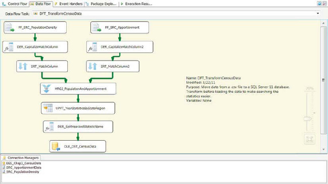
Figure 3-24. DFT_TransformCensusData

FF_SRC_PopulationDensity and FF_SRC_Apportionment, flat file sources, use the same properties as the source components of the HelloWorld package with the exception of the source file. Because the files contain different census data about the same states, we want to combine them into one dataset. The only option to handle this requirement during the extraction is to use a Merge Join component. In order to use this component, the data needs to be sorted by the key values (join columns). SSIS is case and space sensitive, so we have to prepare the join columns before we can sort them. The Derived Column components take care of this for each of the data streams. The Derived Column component creates a new column by evaluating an expression for every row that is passed through the data flow path. The newly created column can be added as a new column, or you can replace an existing column of the same data type in the data flow path.

As shown in Figure 3-25, the Derived Column component uses string functions in order to ensure that the columns from the different flat files match. To add it to the Data Flow, you can double-click the object in the SSIS Toolbox or click and drag it onto the flow. The first thing we suggest that you do after adding it is renaming it using the standards. After adding it to the flow, you must connect the data path to it. After you connect the data path, you can double-click it to open the editor. In the editor, we added the expression UPPER(TRIM(STATE_OR_REGION)) and used the Add as New Column option. We also renamed the column to MatchColumn to capture the purpose of the column.

The top panes allow you to easily reference the available inputs for the derived column as well as the functions that can perform the derivations. The Variables tree displays all the variables that are available to the scope of the data flow that the component belongs to. Because we did not define any variables for this example, the only variables available are the system variables that are a part of all packages. The Columns tree allows you to quickly click and drag the available columns into the expression. The functions are categorized by the different data types they return. With these two reference panes, you can easily start to modify the input with ease.

The TRIM() function removes the leading and trailing spaces of the included string object. Because SSIS will not ignore trailing spaces as SQL Server can be set to do, we need to take extra precautions when joining or looking up with SSIS. The UPPER() function will change the case of the included string object to uppercase. SSIS is also case sensitive, whereas SQL Server has options that can disable this feature. By forcing the column to be in uppercase and generating a new column to hold this uppercase string, we are not actually modifying the original. This will allow us to insert the data into the database as is without alteration. Because this is a Unicode string column, only the Length column is populated; for numeric data types, the precision and scale come into play, and for string data, the code page can be specified. The data will tie together based on the STATE_OR_REGION value, so we have to use this column as the key value later in the pipeline.

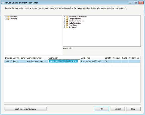
Figure 3-25. Derived column—modifying the match column

The Sort component performs the exact task that the name suggests: it sorts columns in ascending and descending orders. You should rename it as soon as you add it to the data flow. After the data flow path is connected to it from DER_CapitalizeMatchColumn, it can sort multiple columns, each marked by its position in the sort order, as Figure 3-26 demonstrates. There are also options available for the string comparisons performed for the sorting. Because we handled the case and empty space issues through the expression in the derived column, we do not need to worry about the comparison flags. The output alias allows you to rename the sorted column. The columns that are not being sorted are simply marked to be passed through. By checking off columns in this component, we can actually trim the pipeline, but for this particular example, we are looking for all the data present. There is a check box at the bottom that will remove rows with duplicate sort values. This functionality will arbitrarily remove the duplicate record. There is no reason to allow this nondeterministic behavior unless all the columns in the pipeline are being included in the sort; then this feature will allow you to effectively remove your duplicates.

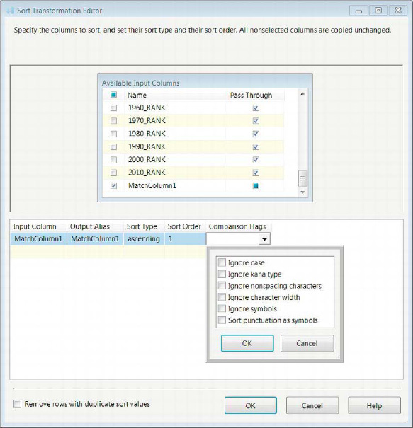
Figure 3-26. Sort Transformation Editor

The Merge Join component in Figure 3-27 brings all the data together. It will utilize the metadata to automatically detect which columns are being sorted and use their sort order to join them. We want to perform an inner join so that only states that are represented in both flat files are passed through. The component supports inner, left, and full outer joins. There is a Swap Inputs button that can add the right join functionality by swapping the outputs pointing to its inputs. The tables in the top half visually represent the left and right inputs. The name of their source is present as the name of the table.

We want only one state name column to pass through, and because we are performing an inner join, it does not matter which input’s state name we use as long as we pick only one of them. We checked off all the columns that are present in the pipeline with the exception of the MatchColumns from both inputs and the right input’s STATE_OR_REGION.

We highly recommend that you trim your pipeline as high up in the data flow as possible. This allows you to use your buffer space on required data only. The output alias allows you to rename each of the columns that the component includes in its output after the join. The Merge Join component has an important property that needs to be set when you include the component in a data flow. The property name is TreatNullsAsEqual. By default it is set to True, but we recommend that you set it to False. There are implications when leaving this property with the default value, mainly the possibility of creating cross join like datasets.

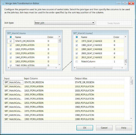
Figure 3-27. Merge Join Transformation Editor

The Unpivot component, whose editor is shown in Figure 3-28, is designed to make denormalized datasets into more-normalized datasets. It works similarly to the UNPIVOT operator in T-SQL. The STATE_OR_REGION column contains the data around which we want to unpivot the rest of the columns as rows. In order make sure that the component ignores the column, we set it to be simply passed through the component. The rest of the columns are passed as inputs to the component. These columns will be unpivoted into rows directly in the data flow path. The Destination Column creates a column to store the statistic that is reported in each column and maintain it as a part of the column as it is turned into a row value. The Pivot Key Value represents the string that will be a part of the dataset to show what the statistic represents. In the text field for Pivot Key Value Column Name, you can name the column that will store the pivot key values. With our dataset, the pivot key represents the combination of the year and the statistic’s name, so we named it YearAndStatisticName.

When you are choosing the columns to pass as inputs to the component, the Pivot Key Value is automatically populated. This default value it takes is the column name itself. You can also define the specific column each pivot key will populate; for our purpose, we require only that all the statistics are populated into one column. A column name is required for the pivot key column.

Figure 3-28. Unpivot Transformation Editor

Because the Pivot Key combines two values, Year and Statistic Name, we utilize a derived column to split that data into two columns. Figure 3-29 demonstrates how we split the column. We add two columns based on the data stored in the YearAndStatisticName column. We use the following expressions to generate the Year and the StatisticName columns, respectively: LEFT(YearAndStatisticName,4) and SUBSTRING(YearAndStatisticName,6,LEN(YearAndStatisticName)).

Because we know that the first four characters of the column value have to be the year, we can use the LEFT() string function to extract the year and store it in a new column named Year. For the statistic name, we have to use the whole string with the exception of the first five characters. The SUBSTRING() string function allows us to define start and end positions of the string. The sixth position is the first character after the underscore, and we want to get the rest of the string, so we use the LEN() string function to define the position of the last character of the string.

Figure 3-29. DER_SplitYearAndStatistics

With the original column split into more-granular data, we can insert this data into a table with the structure defined in Listing 3-3. We used the functionality of the OLE DB destination component to generate create table scripts based on the inputs to generate this script. We removed the column YearAndStatisticName from the create script because it was no longer required. In the mapping of the OLE DB destination component, we ignore the YearAndStatisticName column. The data types of the derived columns are Unicode, but the columns that are sourced from the flat file maintain their code page.

The results of the execution are shown in Figure 3-30. As we discussed earlier, the row count of the output of the Unpivot operator is directly related to the number of distinct records of the ignored columns in relation to the number of columns unpivoted. The Merge Join also omits two records from the left input stream because they are not contained in the Apportionment dataset. The data for the District of Columbia and Puerto Rico is not included in the Apportionment data because these two territories do not have representation in the US Congress. Because we performed an inner join, only data that is common to both sets is allowed to flow further down the pipeline.

Figure 3-30. RealWorld.dtsxexecution

The query in Listing 3-4 shows us the benefits of transforming the data in such a way. Without the Unpivot component, we would have to include all the columns we required in the SELECT clause. With this component, we simply define the proper WHERE clause to see only the data that we require. The denormalized form allows us to include more statistics and more years without having to worry about modifying the table structure to accommodate the new columns.

The query in Listing 3-4 shows us all the statistics for the state of New York in the year 2010. Without the denormalization, we would have to include six columns to account for the year and the different statistics. If we wanted to see all the data for New York since the data collection started, we would have to include 66 columns rather than simply omitting the WHERE clause limiting the year.

Summary

SSIS 11 enables you to extract data from a variety of sources and load them into a variety of destinations. In this chapter, we introduced you to a simple package that extracted the data and loaded it without any transformations. This demonstrated the simplest ETL task that an SSIS 11 package can perform. We then upped the ante and introduced you to a slightly more complex package that transformed the data as it was being extracted. This package demonstrated some of the demands of the real world on ETL processes. We walked you through the process of adding the executables and the components to the package designers. In the next chapter, we will show you all the connection managers available to you in SSIS 11.