A. Trigonometric Identities

(E.1)

(E.2)

(E.3)

(E.4)

(E.5)

(E.6)

(E.7)

(E.8)

(E.9)

B. Series Expansions

(E.10)

(E.11)

(E.12)

(E.13)

(E.14)

(E.15)

(E.16)

(E.17)

(E.18)

(E.19)

C. Some Common Indefinite Integrals

Note: For each of the indefinite integrals, an arbitrary constant may be added to the result.

(E.20)

(E.21)

(E.22)

(E.23)

(E.24)

(E.25)

(E.26)

(E.27)

(E.28)

(E.29)

(E.30)

(E.31)

(E.32)

(E.33)

(E.34)

(E.35)

(E.36)

(E.37)

(E.38)

D. Some Common Definite Integrals

(E.39)

(E.40)

(E.41)

(E.42)

(E.43)

(E.44)

(E.45)

E. Definitions of Some Common Continuous Time Signals

(E.46)

(E.47)

(E.48)

(E.49)

F. Fourier Transforms

Table E.1. Common Fourier transform pairs

Signal (Time Domain)	Transform (Frequency Domain)
rect(t/t0)	t0 sinc(ft0 )
tri(t/t0 )	t0 sinc2 (ft0 )
sinc(t/t0 )	t0 rect(ft0 )
sinc2(t/t0 )	t0 tri(ft0 )
exp(j2πfo t)	δ(f – fo)
cos(2πfo t + θ)
δ(t – to)	exp(−j2πfto)
sgn(t)
u(t)
exp(−(t/t0 )2)

G. z-Transforms

Table E.2. Common z-transform pairs

Signal	Transform	Region of Convergence
δ[n]	1	All z
u[n]		|z| > 1
nu[n]		|z| > 1
n2 u[n]		|z| > 1
n3 u[n]		|z| > 1
bnu[n]		|z| > |b|
nbnu[n]		|z| > |b|
n2bnu[n]		|z| > |b|
bncos[Ωon]u[n]		|z| > |b|
bn sin[Ωon]u[n]		|z| > |b|
		|z| > 1
		|z| > |b|
	exp(bz_1)	All z

H. Laplace Transforms

Table E.3. Common Laplace transform pairs

Function	Transform	Region of Convergence
u(t)	1/s	Re[s]>0
exp(−bt)u(t)		Re[s]>-b
sin (bt)u(t)		Re[s] >0
cos(bt)u(t)		Re[s] >0
e− at sin(bt)u(t)		Rs[s] >-a
e− at cos(bt)u(t)		Rs[s] >-a
δ(t)	1	All s
	s	All s
tnu(t), n > 0		Re[s] >0
tne−btu(t), n ≥ 0		Re[s] >-b

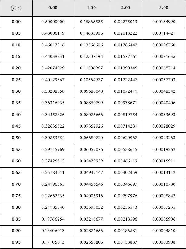
I. Table of the Q-function

The following table lists values of the function Q(x) for 0 ≤ x ≤ 4 in increments of 0.05. To find the appropriate value of x, add the value at the beginning of the row to the value at the top of the column. For example, to find Q (1.75), find the entry from the column headed by 1.00 and the row headed by 0.75 to get Q (1.75) = 0.04005916.

Table E.4. Values of Q(x) for 0 ≤ x ≤ 4 (in increaments of 0.05)