8.3 UMTS Channel Simulator

This section presents the design and implementation procedure for a multimedia evaluation testbed of the UMTS forward link. A WCDMA physical link layer simulator has been implemented using the Signal Processing WorkSystem (SPW) software simulation tools developed by Cadence Design System Inc. [27]. The model has been developed in a generic manner that includes all the forward link radio configurations, channel structures, channel coding/decoding, spreading/de-spreading, modulation parameters, transmission modeling, and their corresponding data rates according to the UMTS specifications. The performance of the simulator model is validated by comparison with figures presented in the relevant 3GPP documents [28], [29] for the specified measurement channels, propagation environments, and interference conditions in [30]. Using the developed simulator, a set of UMTS error pattern files is generated for different radio bearer configurations in different operating environments, and the results are presented. Furthermore, UMTS link-level performance is enhanced by implementing a closed-loop power-control algorithm. A UMTS radio interface protocol model, which represents the data flow across the UMTS protocol layers, is implemented in Visual C++. It is integrated with the physical link layer model to emulate the actual radio interface experienced by users. This allows for interactive testing of the effects of different parameter settings of the UMTS Terrestrial Radio Access Network (UTRAN) upon the received multimedia quality.

8.3.1 UMTS Terrestrial Radio Access Network (UTRAN)

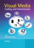
The system components of UTRAN are shown in Figure 8.22. Functionally, the network elements are grouped into the radio network subsystem (RNS), the core network (CN), and the user equipment (UE). UTRAN consists of a set of RNSs connected to the core network through the Iu interface. The interface between the UE and the RNS is named Uu. An RNS contains a radio network controller (RNC) and one or more node Bs. The RNS handles all radio-related functionality in its allocated region. A node B is connected to an RNC through the Iub interface, and communication between RNSs is conducted through the Iur interface. One or more cells are allocated to each node B.

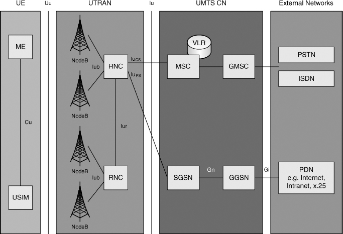
Figure 8.22 Systems components in a UMTS

The protocol within the CN is adopted from the evolution of GPRS protocol design. However, both the UE and UTRAN feature completely new protocol designs, which are based on the new WCDMA radio technology. WCDMA air interfaces have two versions, defined for operation in frequency division duplexing (FDD) and time division duplexing (TDD) modes. Only the FDD operation is investigated in this chapter. The modulation chip rate for WCDMA is 3.8 mega chips per second (Mcps). The specified pulse-shaping roll-off factor is 0.22. This leads to a carrier bandwidth of approximately 5 MHz. The nominal channel spacing is 5 MHz. However, this can be adjusted approximately between 4.4 and 5 MHz, to optimize performance depending on interference between carriers in a particular operating environment. As described in Table 8.13, the FDD version is designed to operate in either of the following frequency bands [30]:

• 1920–1980 MHz for uplink and 2110–2170 MHz for downlink.
• 1850–1950 MHz for uplink and 1930–1990 MHz for downlink.

Table 8.13 WCDMA air interface parameters for FDD-mode operation

Operating Frequency Band	2110–2170 MHz 1930–1990 MHz downlink 1920–1980 MHz 1850–1910 MHz uplink
Duplexing Mode	Frequency Division Duplex (FDD)
Chip Rate	3.84 mega chips per second
Pulse-shaping Roll-off Factor	0.22
Carrier Bandwidth	5 MHz

All radio channels are code-division multiplexed and are transmitted over the same (entire) frequency band.

WCDMA supports highly variable user data rates with the use of variable spreading factors, thus facilitating the bandwidth-on-demand concept. Transmission data rates of up to 384 kbps are supported in wide-area coverage, and 2 Mbps in local-area coverage. The radio frame length is fixed at 10 ms. The number of information bits or symbols transmitted in a radio frame may vary, corresponding to the spreading factor used for the transmission, while the number of chips in a radio frame is fixed at 38 400 [30].

8.3.1.1 Radio Interface Protocol

The radio interface protocol architecture, which is visible in the UTRAN and the user equipment (UE), is shown in Figure 8.23. Layer 1 (L1) comprises the WCDMA physical layer. Layer 2 (L2), which is the data-link layer, is further split into medium access control (MAC), radio link control (RLC), packet data convergence protocol (PDCP), and broadcast multicast control (BMC). The PDCP exists mainly to adapt packet-switched connections to the radio environment by compressing headers with negotiable algorithms. Adaptation of broadcast and multicast services to the radio interface is handled by BMC. For circuit-switched connections, user-plane radio bearers are directly connected to the RLC. Every radio bearer should be connected to one unique instance of the RLC.

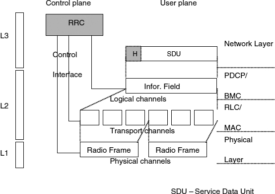
Figure 8.23 Radio-interface protocol architecture

The radio resource control (RRC) is the principal component of the network layer – layer 3 (L3). This comprises functions such as broadcasting of system information, radio resource handling, handover management, admission control, and provision of requested QoS for a given application. Unlike the traditional layered protocol architecture, where protocol layer interaction is only allowed between adjacent layers, RRC interfaces with all other protocols, providing fast local interlayer controls. These interfaces allow the RRC to configure characteristics of the lower-layer protocol entities, including parameters for the physical, transport, and logical channels [31]. Furthermore, the same control interfaces are used by the RRC layer to control the measurements performed by the lower layers, and by the lower layers to report measurement results and errors to the RRC. See Figure 8.24.

UTRAN supports both circuit-switched and packet-switched connections. In order to transmit an application's data between UE and the end system, QoS-enabled bearers have to be established between the UE and the media gateway (MGW). Figure 8.25 shows the user plane protocol stack used for data transmission over packet-switched connection in Release 4.

Figure 8.24 Interactions between RRC and lower layers [32]. Reproduced, with permission, from 3GPP TS 25.301, “Radio interface protocol architecture”, Release 4, V4.4.0. (2002–09). ©2002 3GPP. ©1998 3GPP. Reproduced by permission of © European Telecommunications Standards Institute 2008. Further use, modification, redistribution is strictly prohibited. ETSI standards are available from http://pda.etsi.org/pda/

Figure 8.25 User plane UMTS protocol stack for packet-switched connection [6]. Reproduced, with permission, from “Technical specification, 3rd Generation Partnership Project; technical specification group services and systems aspects; general packet radio service (GPRS); service description stage 2 (release 4)”, 3GPP TS 23.060 V4.0.0, March 2001. ©2001 3GPP. ©1998 3GPP. Reproduced by permission of © European Telecommunications Standards Institute 2008. Further use, modification, redistribution is strictly prohibited. ETSI standards are available from http://pda.etsi.org/pda/

8.3.1.2 Channel Structure

Channels are used as a means of interfacing the L2 and L1 sub-layers. Between the RLC/MAC layer and the network layer, logical channels are used. Between the RLC/MAC and the PHY layers, the transport channels are used, and below the PHY layer is the physical channel (see Figure 8.23).

Generally, logical channels can be divided into control and traffic channels. The paging control channel and the broadcast control channel are for the downlink only. The common control channel is a bi-directional channel shared by all UEs, while the common transport channel is a downlink-only shared channel. Dedicated control channels and dedicated transport channels are unique for each UE.

Transport channels are used to transfer the data generated at a higher layer to the physical layer, where it gets transmitted over the air interface. The transport channels are described by a set of transport channel parameters, which are designed to characterize the data transfer over the radio interface. Each transport channel is accompanied by the transport format indicator (TFI), which describes the format of data to be expected from the higher layer at each time interval. The physical layer combines the TFI from multiple transport channels to form a transport format combination indicator (TFCI). This facilitates the combination of several transport channels into a composite transport channel at the physical layer, as shown in Figure 8.26, and their correct recovery at the receiver [31].

In UTRA, two types of transport channel exist, namely dedicated channel and common channel. As the names suggest, the main difference between them is that a common channel has its resources divided between all or a group of users in a cell, while a dedicated channel reserves resources for a single user.

Figure 8.26 Transport channel mapping

The transmission time interval (TTI) defines the arrival period of data from higher layers to the physical layer. TTI size has been defined to be 10, 20, 40, and 80 ms. Selection of TTI size depends on the traffic characteristics. The amount of data that arrives in each TTI can vary in size, and is indicated in the transport format indicator (TFI). In the case of transport channel multiplexing, TTIs for different transport channels are time-aligned, as shown in Figure 8.27.

The physical channels are defined by a specific set of radio interface parameters, such as scrambling code, spreading code, carrier frequency, and transmission power step. The channels are used to convey the actual data through the wireless link. The most important control information in a cell is carried by the primary common control physical channel (PCCPCH) and secondary common control physical channel (SCCPCH). The difference between these two is that the PCCPCH is always broadcast over the whole cell in a well-defined format, while the SCCPCH can be more flexible in terms of transmission diversity and format. In the uplink, the physical random access channel (PRACH) and physical common packet channel (PCPCH) are data channels shared by many users. The slotted ALOHA approach is used to grant user access in PRACH [33]. A number of small preambles precede the actual data, serving as power control and collision detection. The physical downlink shared channel (PDSCH) is shared by many users in downlink transmission. One PDSCH is allocated to a single UE within a radio frame, but if multiple PDSCHs exist they can be allocated to different UEs arbitrarily: one to many or many to one. The dedicated physical data channel (DPDCH) and dedicated physical control channel (DPCCH) together realize the dedicated channel (DCH), which is dedicated to a single user [31].

Figure 8.27 Transmission time intervals (TTIs) in transport channel multiplexing

8.3.1.3 Modes of Connection

Figure 8.28 shows the possible modes of realizing the connections of the radio bearers at each layer. PDCP, RLC and MAC modes must be combined with physical-layer parameters in a way that satisfies different QoS demands on the radio bearers. However, the exact parameter setting is a choice of the implementer of the UMTS system and of the network operator.

The radio bearer can be viewed as either packet switched (PS) or circuit switched (CS). A PS connection passes the PDCP, where header compression can be applied or not. The RLC offers three modes of data transfer. The transparent mode transmits higher-layer payload data units (PDUs) without adding any protocol information and is recommended for real-time conversational applications. The unacknowledged mode will not guarantee the delivery to the peer entity, but offers other services such as detection of erroneous data. The acknowledged mode guarantees the delivery through the use of automatic repeat request (ARQ) [34].

Figure 8.28 Interlayer modes of operation

The MAC layer can be operated in dedicated, shared, or broadcast mode. Dedicated mode is responsible for handling dedicated channels allocated to a UE in connected mode, while shared mode takes the responsibility of handling shared channels. The broadcast channels are transmitted using broadcast mode. The physical layer follows the MAC in choosing a dedicated or shared physical channel [35].

In UTRA, spreading is based on the orthogonal variable spreading factor (OVSF) technique. Quadrature phase shift keying (QPSK) modulation is used for downlink transmission. Both convolutional and turbo coding are supported for channel protection. The maximum possible transmission rate in downlink is 5760 kbps. It is provided by three parallel codes with a spreading factor of 4. With 1/2 rate channel coding, this could accommodate up to 2.3 Mbps user data. However, the practical maximum user data rate is subject to the amount of interference present in the system and the quality requirement of the application.

8.3.2 UMTS Physical Link Layer Model Description

The physical link layer parameters and the functionality of the downlink for the FDD mode of the UMTS radio access scheme are described in this subsection. The main issues addressed are transport/physical channel structures, channel coding, spreading, modulation, transmission modeling, and channel decoding. Only the dedicated channels are considered, as the end application is real-time multimedia transmission for dedicated users. The implementation closely follows the relevant 3GPP specifications. A closed-loop fast power control method is also implemented.

The developed model simulates the UMTS air interface. Figure 8.29 is a block diagram of the simulated physical link layer. It can be seen that the transmitted signal is subjected to a multipath fast-fading environment, for which the power-delay profiles are specified in [36]. In addition, an AWGN source is presented after the multipath propagation model. Cochannel interferers are not explicitly presented in the model because the loss of orthogonality of co-channels due to multipath propagation can be quantified using a parameter called the “orthogonality factor” [31], which indicates the fraction of intra-cell interfering power that is perceived by the receiver as Gaussian noise. The multipath-induced intersymbol interference is implicit in the developed chip-level simulator. By changing the variance of the AWGN source, the bit error and block error characteristics can be determined for a range of carrier-to-interference (C/I) ratios and Signal-to-Noise (S/N) ratios for different physical layer configurations. The simulator only considers a static C/I and S/N profile, and no slow fading effects are implemented. However, slow fading can easily be implemented by concatenating the data sets describing the channel bit error characteristics of different, static, C/I levels.

Each radio access bearer (RAB) is normally accompanied by a signaling radio bearer (SRB) [37]. Therefore, in the simulator, two dedicated transport channels are multiplexed and mapped on to a physical channel.

8.3.2.1 Channel Coding

UTRA employs four channel-coding schemes, offering flexibility in the degree of protection, coding complexity, and traffic capacity available to the user. The available channel-coding methods and code rates for dedicated channels are 1/2 rate convolutional code, 1/3 rate convolutional code, 1/3 rate turbo code, and no coding.

Figure 8.29 UMTS physical link layer model

1/2 rate and 1/3 rate convolution coding is intended to be used with low data rates, equivalent to the data rates provided by second-generation cellular networks [31]. For high data rates, 1/3 rate turbo coding is recommended, and it typically brings performance benefits when sufficiently large input block sizes are achieved. The channel-coding schemes are defined in [38], and are outlined here.

Convolutional Coding

Convolutional codes with constraint length 9 and coding rates 1/3 and 1/2 are defined. Channel code block size is varied according to the data bit rates. The specified maximum code block size for convolutional coding is 504. If the number of bits in a transmission time interval (TTI) exceeds the maximum code block size then code block segmentation is performed (Figure 8.30). In order to achieve similar size code blocks after segmentation, filler bits are added to the beginning of the first block.

Figure 8.30 Example of block segmentation at the channel encoder

Eight tail bits with binary value 0 are added to the end of the code block before encoding, and initial values of the shift register are set to 0s when the encoding is started. The generator polynomials used in the encoding as given in [38] are:

Rate 1/2 convolutional coder:

Rate 1/3 convolutional coder:

Note that the UTRA uses two different sets of generator polynomials to achieve two different convolutional code rates. If K_i denotes the number of bits in the ith code block before encoding then the number of bits after encoding, Y_i, is:

Y_i = 2K_i + 16 with 1/2 rate coding.

Y_i = 3K_i + 24 with 1/3 rate coding.

Turbo Coding

Turbo codes employ two or more error control codes, which are arranged in such a way as to enhance the coding gain. They have been demonstrated to closely approach the Shannon capacity limit on both AWGN and Rayleigh fading channels. Traditionally, two parallel or serial concatenated recursive convolutional codes are used in the encoder implementation. A bit interleaver is used in between the encoders. Generated parity bitstreams from two encoders are finally multiplexed to produce the output turbo-coded bitstream. Turbo decoding is carried out iteratively. The whole process results in a code that has powerful error-correction properties.

The defined turbo coder for use in UMTS is a parallel-concatenated convolutional code with two eight-state constituent encoders and one turbo-code internal interleaver. The coding rate of the turbo coder is 1/3. Figure 8.31 shows the configuration of the turbo coder.

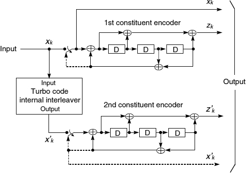
Figure 8.31 Structure of rate 1/3 turbo coder [38]. Reproduced, with permission, from “3rd Generation Partnership Project; technical specification group radio access network; multiplexing and channel coding (FDD) (release 4)”, 3GPP TS 25.212 V4.6.0 (2002–09). ©2002 3GPP. ©1998 3GPP. Reproduced by permission of © European Telecommunications Standards Institute 2008. Further use, modification, redistribution is strictly prohibited. ETSI standards are available from http://pda.etsi.org/pda/

The transfer function of the eight-state constituent code is defined as:

where:

The initial values of the shift registers are set to 0s at the start of the encoding. Output from the turbo code is read as X₁, Z₁, Z′₁, and so on. Termination of the turbo coder defined in UMTS is performed in a different way to conventional turbo code termination, which uses 0 incoming bits to generate the trellis termination bits. Here, the shift register feedbacks after all information bits have been encoded are used to generate the termination bits. To terminate the first constituent encoder, switch A in Figure 8.31 is set to the lower position while the second constituent encoder is disabled. Likewise, the second constituent encoder is terminated by setting switch B in Figure 8.31 to the lower position while the first constituent encoder is disabled.

The turbo code internal interleaver arranges incoming bits into a matrix. If the number of incoming bits is less than the number of bits that the matrix could contain, padding bits are used. Then intra-row and inter-row permutations are performed according to the algorithm given in [38]. Pruning is performed at the output, so the output block size is guaranteed to be equal to the input block size. If K_i denotes the number of input bits in a code block, the number of turbo code output bits Y_i, is Y_i = 3K_i + 12 for 1/3 code rate.

The minimum block size and the maximum block size for turbo coding are defined as 40 bits and 5114 bits respectively. Data sizes below 40 bits can be coded with turbo codes; however, in such a case, dummy bits are used to fill the 40 bit minimum-size interleaver. If the incoming block size exceeds the maximum size then segmentation is performed before channel coding.

8.3.2.2 Rate Matching

Rate matching is used to match the incoming data bits to available bits on the radio frame. Rate matching is achieved either by bit puncturing or by repetition. If the amount of incoming data is larger than the number of bits that can be accommodated in a single frame then bit puncturing is performed. Otherwise, bit repetition is performed. In the case of transport channel multiplexing, rate matching should take into account the number of bits arriving in other transport channels.

The rate matching algorithm depends on the channel coding applied. The corresponding rate matching algorithms for convolutional and turbo coding are defined in [38]. In the simulation under discussion, rate matching is only performed for the signaling bearer. As signaling data is protected using convolutional codes, the rate matching algorithm is implemented only for convolutional coding.

8.3.2.3 Interleaving

In UTRA, data interleaving is performed in two steps: first and second interleaving. These are also known as inter-frame interleaving and intra-frame interleaving, respectively. The first interleaving is a block interleaver with inter-column permutations (inter-frame permutation) and is used when the delay budget allows more than 10 ms of interleaving. In other words, the specified transmission time interval (TTI), which indicates how often data comes from higher layers to the physical layer, is larger than 10 ms. The TTI is directly related to the interleaving period and can take values of 10, 20, 40 or 80 ms. Table 8.14 shows the inter-column permutation patterns for first interleaving. Each column contains data bits for 10 ms duration.

The second or intra-frame interleaving performs data interleaving within a 10 ms radio frame. This is also a block interleaver with inter-column permutations applied. Incoming data bits are input into a matrix with n rows and 30 columns, row by row with a starting position of column 0 and row 0. The number of rows is the minimum integer n, which satisfies the condition:

Table 8.14 Inter-columns permutation patterns for first interleaving [38]. Reproduced, with permission, from “3rd Generation Partnership Project; technical specification group radio access network; multiplexing and channel coding (FDD) (release 4)”, 3GPP TS 25.213 V4.3.0. (2002–06). ©2002 3GPP. ©1998 3GPP. Reproduced by permission of © European Telecommunications Standards Institute 2008. Further use, modification, redistribution is strictly prohibited. ETSI standards are available from http://pda.etsi.org/pda/

Table 8.15 Inter-columns permutation patterns for second interleaving [38]. Reproduced, with permission, from “3rd Generation Partnership Project; technical specification group radio access network; multiplexing and channel coding (FDD) (release 4)”, 3GPP TS 25.213 V4.3.0. (2002–06). ©2002 3GPP. ©1998 3GPP. Reproduced by permission of © European Telecommunications Standards Institute 2008. Further use, modification, redistribution is strictly prohibited. ETSI standards are available from http://pda.etsi.org/pda/

Number of columns	Inter-column permutation patterns
30	<0,20,10,5,15,25,3,13,23,8,18,28,1,11,21,6,16,26,4,14,24,19,9,29,12,2,7,22,27,17>

Total number of bits in radio block ≤ n × 30

If the total number of bits in the radio block is less than that, it is necessary to fill the whole matrix, and bit padding is performed. The inter-column permutation for the matrix is performed based on the pattern shown in Table 8.15. Output is read out from the matrix column by column, and finally pruning is performed to remove padding bits that were added to the input of the matrix before the inter-column permutation.

8.3.2.4 Spreading and Scrambling

The spreading in the downlink is based on the channelization codes and is used to preserve the orthogonality among different downlink physical channels within one cell (or sector of a cell), and to spread the data to the chip rate, which is 3.84 Mcps. In UTRA, spreading is based on the orthogonal variable spreading factor (OVSF) technique. The OVSF code tree is illustrated in Figure 8.32.

Typically only one OVSF code tree is used per cell sector in the base station (or node B). The common channels and dedicated channels share the same code tree resources. The codes are normally picked from the code tree; however, there are certain restrictions as to which of the codes can be used for a downlink transmission. A physical channel can only use a certain code from the tree if no other physical channel is using a code that is on an underlying branch. Neither can a smaller spreading factor code on the path to the root of the tree be used. This is because even though all codes from the same level are orthogonal to each other, two codes from different levels are orthogonal to each other only if one of them is not the mother code of the other. The radio network controller in the network manages the downlink orthogonal codes within each base station.

The spreading factor on the downlink may vary from 4 to 512 (an integer power of 2), depending on the data rate of the channel. Table 8.16 summarizes the channel bit rates, data rates, and spreading factors for downlink dedicated physical channels.

In addition to spreading, a scrambling operation is performed in the transmitter. This is used to separate base stations (cell sectors) from one another. As the chip rate is already achieved with spreading, the symbol rate is not affected by scrambling. The downlink scrambling uses the Gold codes [39]. The number of primary scrambling codes is limited to 512, simplifying the cell search procedure. The secondary scrambling codes are used in the case of beam-steering and adaptive antenna techniques [40].

Figure 8.32 Example of OVSF code tree used for downlink

8.3.2.5 Modulation

Quadrature phase shift keying (QPSK) modulation is applied on time-multiplexed control and data streams on the downlink. Each pair of consecutive symbols is serial-to-parallel converted and mapped on to I and Q branches. The symbols on I and Q branches are then spread to the chip rate by the same real-valued channelization code. The spread signal is then scrambled by a cell-specific complex-valued scrambling code.

Table 8.16 Downlink dedicated channel bit rates

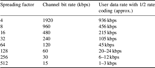
Figure 8.33 Downlink modulation [39]. Reproduced, with permission, from “3rd Generation Partnership Project; technical specification group radio access network; spreading and modulation (FDD) (release 4)”, 3GPPTS 25.213 V4.3.0. (2002–06). ©2002 3GPP. ©1998 3GPP. Reproduced by permission of © European Telecommunications Standards Institute 2008. Further use, modification, redistribution is strictly prohibited. ETSI standards are available from http://pda.etsi.org/pda/

Figure 8.33 shows the spreading and modulation procedure for a downlink physical channel. A square-root raised cosine filter with a roll-off factor of 0.22 is employed for pulse shaping, and the pulsed shaped signal is subsequently up-converted and transmitted.

8.3.2.6 Physical Channel Mapping

The frame structure for a downlink dedicated physical channel is shown in Figure 8.34. Each radio frame has 15 equal-length slots. The slot length is 2560 chips. As shown in Figure 8.34, the DPCCH and DPDCH are time-multiplexed within the same slot [41].

Each slot consists of pilot symbols, transmit power control (TPC) bits, transport format combination indicator (TFCI) bits, and bearer data. The number of information bits transmitted in a single slot depends on the source data rates, the channel coding used, the spreading factor, and the channel symbol rate. The exact number of bits in the downlink DPCH fields is given in [41] and is summarized in Table 8.17.

8.3.2.7 Propagation Model

The channel model used in the simulator is the multipath propagation model specified by IMT2000 in [36]. This model takes into account that the mobile radio environment is dispersive, with several reflectors and scatterers. For this reason, the transmitted signal may reach the receiver via a number of distinct paths, each having different delays and amplitudes. The multipath fast fading is modeled by the superposition of multiple single-faded paths with different arrival times and different average powers for specified power-delay profiles in [36]. Each path is characterized by Rayleigh distribution (first-order statistic) and classic Doppler spectrum (second-order statistic).

Figure 8.34 Frame structure for downlink DPCH

Table 8.17 DPDCH and DPCCH fields (3GPP TS 25.211). Reproduced, with permission, from “3rd Generation Partnership Project; technical specification group radio access network; physical channels and mapping of transport channel on to physical channel (FDD) (release 4)”, 3GPP TS 25.211 V4.6.0. (2002–09). ©2002 3GPP. ©1998 3GPP. Reproduced by permission of © European Telecommunications Standards Institute 2008. Further use, modification, redistribution is strictly prohibited. ETSI standards are available from http://pda.etsi.org/pda/

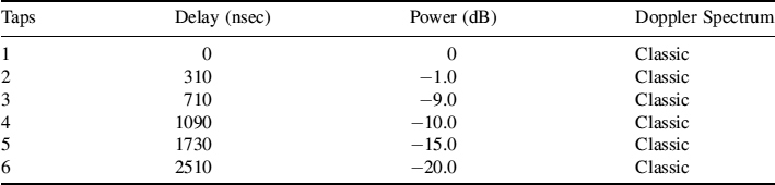
Figure 8.35 shows a block diagram of a four-path frequency selective fading channel. UTRAN defines three different multipath power-delay profiles for use in different propagation environments. There are indoor office environments, outdoor-to-indoor and pedestrian environments, and vehicular environments. All of these models are implemented in the simulator and the tapped-delay line parameters for the vehicular environment are shown in Table 8.18. Mobile channel impulse response is updated 100 times for every coherence time interval.

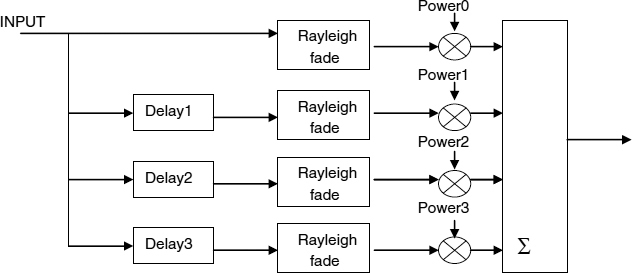
Figure 8.35 Four-path frequency selective fading channel

Table 8.18 Vehicular A test environment [36]. Reproduced, with permission, from “Universal Mobile Telecommunications System (UMTS); selection procedures for the choice of radio transmission technologies of the UMTS (UMTS 30.03 version 3.2.0)”, TR 101 112 V3.2.0 (1998–04) ©1998 3GPP. ©1998 3GPP. Reproduced by permission of © European Telecommunications Standards Institute 2008. Further use, modification, redistribution is strictly prohibited. ETSI standards are available from http://pda.etsi.org/pda/

After the multipath channel shown in Figure 8.29, white Gaussian noise is added to simulate the effect of overall interference in the system, including thermal noise and inter-cell interference.

8.3.2.8 Rake Receiver

The rake receiver is a coherent receiver that attempts to collect the signal energy from all received signal paths that carry the same information. The rake receiver therefore can significantly reduce the fading caused by these multiple paths.

The operation of the rake receiver follows three main operating principles (see Figure 8.36). The first is the identification of the time-delay positions at which significant energy arrives, and the time alignment of rake fingers for combining. The second is the tracking of fast-changing phase and amplitude values originating from the fast-fading process within each correlation receiver, and the removal of these from the incoming data. Finally, the demodulated and phase-adjusted symbols are combined across all active fingers and passed to the decoder for further processing. The combination can be processed using three different methods:

Figure 8.36 Block diagram of a rake receiver

• Equal gain combining (EGC), where the output from each finger is simply summed with equal gain.
• Maximal ratio combining (MRC), where finger outputs are scaled by a gain proportional to the square root of the SNR of each finger before combining [42]. In this case, the finger output with the highest power dominates in the combination.
• Selective combining (SC), where not all finger outputs are considered in the combination, but some fingers are selected for combining according to the received power on each.

Two types of rake receiver have been developed for the downlink:

1. Ideal rake receiver.
2. Quasi-ideal rake receiver.

The following subsections provide details of the designs of these rake receivers.

Ideal Rake Receiver

The block diagram of an ideal rake receiver is shown in Figure 8.37. Here, perfect channel estimation and perfect finger time alignment is assumed. This is implemented by storing all the fast-fading channel coefficients as a complex vector, where the vector length equals the number of frequency selective fading paths. This vector is then fed from the channel directly to the ideal receiver. At the receiver, the coefficients for each path are first separated and then applied to each rake finger, after being time-aligned in accordance with the delay (from channel delay profile) in each reflected path. Of the three rake finger combination methods, EGC is selected for the ideal receiver as it gives the optimal performance in the presence of ideal channel estimation and perfect time alignment.

Quasi-ideal Rake Receiver

The quasi-ideal rake receiver resembles a practical rake receiver in terms of implementation. However, as depicted in Figure 8.38, ideal finger search for the rake receiver is assumed. That is, each finger in the receiver is assumed to have perfect synchronization with the corresponding path in the channel. First the received data is time-aligned according to the channel delay profile. Then the data on each finger undergoes a complex correlator process to remove the scrambling and spreading codes. As in an actual receiver implementation, pilot bits are used to estimate the momentary channel state for a particular finger. Channel estimation is achieved through the use of a matched filter, which is employed only during the period in which the pilot bits are being received. The pilot bits are sent in every transmit time slot; therefore, the maximum effective channel updating interval is equivalent to half a slot. Output from the matched filter is further refined by using a complex FIR filter. Here, the weighted multislot averaging (WMSA) technique proposed in [43] is employed to reduce the noise variance, and also to track fast channel variation between consecutive channel estimates. Two different sets of weighting for the WSMA filter are used for low vehicular speeds and high vehicular speeds respectively. This is because the limiting factor in channel estimation errors at low vehicular speed is the channel noise rather than the channel variation. Therefore, the noise averaging effect is more desirable at low vehicle speed. By comparison, at high vehicle speed channel variation becomes the limiting factor, hence weighting based on interpolation should be considered. The WMSA technique requires a delay of an integer number of time slots for the channel processing. The time-varying channel effect is removed from the de-scrambled and de-spread signal before it is sent to the signal combiner. MRC is used for the rake finger combination as it gives better performance. Intersymbol interference due to the multipath is implicit in the resulting output.

Figure 8.37 Ideal rake receiver

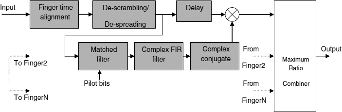
Figure 8.38 Qausi-ideal rake receiver

8.3.2.9 Channel Decoding

In the implementation, a soft-decision Viterbi algorithm is used for the decoding of the convolutional codes. Turbo decoding is based on the standard LogMap algorithm (which is provided in SPW), which tries to minimize the bit error ratio rather than the block error ratio [42]. Eight iterations are performed.

8.3.3 Model Verification for Forward Link

The theoretical formula for the BER probability with an order L MRC diversity combiner is given in [44], and is stated as:

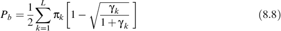
where P_b is the bit error probability, L denotes the number of diversity path, and γ_k is the mean E_b/η for kth diversity path. π_k is given by:

If the rake receiver is assumed to behave as an order L MRC diversity combiner, Equation (8.9) gives the lower bound of the BER performance. Other test conditions assumed in Equation (8.9) are:

• Perfect channel estimation.
• No intersymbol interference presence.
• Each propagation path has a Rayleigh envelope.

Using Equation (8.9), the theoretical lower bound of the performance for the power delay profile that is specified in the case 3 outdoor performance measurement test environment in annex B [30] is calculated. It is depicted in Figure 8.39. Here, a mean SNR value for each individual path is calculated from the global E_b/N_o by simply multiplying it by the fraction of power carried by each path (given in power delay profile). The number of rake fingers equals the number of propagation paths, which is four in this case.

Figure 8.39 Performance of uncoded channel

Figure 8.39 shows the performance in terms of raw BER (uncoded) for varying spreading factors in the above-described test environment. A single active connection is considered. The dashed lines show the performance obtained by Olmos and Ruiz in [44] for similar test conditions. Figure 8.39 clearly illustrates the close match of results obtained from the described model to those given in [44]. As the spreading factor reduces, the performance deviates from that of the theoretical bound, due to the presence of intersymbol interference.

For non-ideal channel estimation, raw BER performance (see Figure 8.40) deviates considerably from the ideal channel estimation performance. Performance degradation is about 3–4 dB for operation at lower E_b/N_o, and increases gradually as E_b/N_o increases. It should be emphasized here that the channel-coding algorithm can correct almost all of the channel error occurrences if the raw BER values are less than 10⁻². Therefore, the region that is interesting for multimedia applications is limited to the top-left-hand corner in Figure 8.40.

8.3.3.1 Model Performance Validation

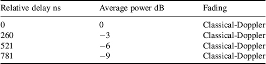
Reference performance figures for the downlink dedicated physical channels are given in [30]. These allow for the setting of reference transmitter and receiver performance figures for nominal error ratios, sensitivity levels, interference levels, and different propagation conditions. Reference measurement channel configurations are specified in Annex A [30], while the reference propagation conditions are specified in Annex B [30]. A mechanism to simulate the interference from other users and control channels in the downlink (named orthogonal channel noise simulator (OCNS)) on the dedicated channel is shown in Annex C [30]. The performance requirements are given in terms of block error ratio (BLER) for different multipath propagation conditions, data rates (hence spreading factors), and channel coding schemes. For example, Table 8.19 lists the required upper bound of BLER for the reference parameter setting shown in Table 8.20. The power-delay profile of the multipath fading propagation condition used in the reference test is given in Table 8.21. Physical channel parameters, transport channel parameters, channel coding, and channel mapping for the 64 kbps reference test channel are depicted in Figure 8.41. As in a typical operating scenario, two transport channels, the data channel and the signaling channel, are multiplexed and mapped on to the same physical channel.

Figure 8.40 Comparison of ideal and non-ideal channel estimate performance

Table 8.19 BLER performance requirement [30]. Reproduced, with permission, from “3rd Generation Partnership Project; technical specification group radio access network; user equipment (UE) radio transmission and reception (FDD) (release 4)”, 3GPP TS 25.101 V410.0 (2002–03). ©2004 3GPP. ©1998 3GPP. Reproduced by permission of © European Telecommunications Standards Institute 2008. Further use, modification, redistribution is strictly prohibited. ETSI standards are available from http://pda.etsi.org/pda/

Table 8.20 Reference parameter setting [30]. Reproduced, with permission, from “3rd Generation Partnership Project; technical specification group radio access network; user equipment (UE) radio transmission and reception (FDD) (release 4)”, 3GPP TS 25.101 V410.0 (2002–03). ©2004 3GPP. ©1998 3GPP. Reproduced by permission of © European Telecommunications Standards Institute 2008. Further use, modification, redistribution is strictly prohibited. ETSI standards are available from http://pda.etsi.org/pda/

Table 8.21 Power-delay profile for case 3 test environment [30]. Reproduced, with permission, from “3rd Generation Partnership Project; technical specification group radio access network; user equipment (UE) radio transmission and reception (FDD) (release 4)”, 3GPP TS 25.101 V410.0 (2002–03). ©2004 3GPP. ©1998 3GPP. Reproduced by permission of © European Telecommunications Standards Institute 2008. Further use, modification, redistribution is strictly prohibited. ETSI standards are available from http://pda.etsi.org/pda/

8.3.3.2 Calculation of E_b/N_o and DPCH_E_C/I_or

Reference test settings are given in terms of the ratio of energy per chip to the total transmit power spectral density of the node B antenna connector. The relationship between E_b/N_o and the setting of the variance σ of the AWGN source and the conversion of DPCH_E_c/I_or to E_b/N_o is given in Equations (8.10) and (8.11) respectively. The derivations of these equations are given in Appendix A.

Figure 8.41 Channel coding of DL reference measurement channel (64 kbps) [30]. Reproduced, with permission, from “3rd Generation Partnership Project; technical specification group radio access network; user equipment (UE) radio transmission and reception (FDD) (release 4)”, 3GPP TS 25.101 V4.10.0. (2002–03). ©2004 3GPP. ©1998 3GPP. Reproduced by permission of © European Telecommunications Standards Institute 2008. Further use, modification, redistribution is strictly prohibited. ETSI standards are available from http://pda.etsi.org/pda/

Table 8.22 Performance validation for convolutional code use

where R_C and R_b are the chip rate and the channel bit rate respectively, and ch_os denotes the channel over sampling factor. Equation (8.11) is equivalent to the equation proposed by Ericsson in [28].

8.3.3.3 UMTS DL Model Verification for Convolutional Code Use

Reference interference performance figures [30] for convolutional code with 12.2 kbps data were compared to the results obtained using the designed simulation model, which is referred to as the CCSR model. A comparison is given in Table 8.22. The reference results are given in terms of the upper bound of the average downlink power, which is needed to achieve the specified block error ratio value.

The results listed in Table 8.22 show that the CCSR model performance is within the performance requirement limits in all propagation conditions. The performance requirements specified in 3GPP are limited to a single value, which is insufficient to test the model performance over a range of propagation conditions. Therefore, performance tests were carried out for a range of DPCH_E_c/I_or for different reference propagation environments, and the results are compared to those obtained by Ericsson [28] and NTT DoCoMo [29]. These results are shown in Figure 8.42.

Figure 8.42 clearly illustrates the close performance of the CCSR model to the results given in the above references. BLER curves for case 1 and case 3 are virtually identical to those given in the above references. In the case 2 propagation environment, the CCSR model outperforms the other two reference figures. The reason for this may be the use of an EGC rake receiver in the CCSR model. Case 2 represents an imaginary radio environment, which consists of three paths with large relative delays and equal average power. Use of EGC in this environment combines energy from all three paths with equal gain, resulting in maximum power output, and shows optimal performance. The path combiner structures used in the reference models are unknown. Performance over AWGN environment shows slight variation at low-quality channels. However, the performance gets closer to that of the reference figure when the channel quality gets better.

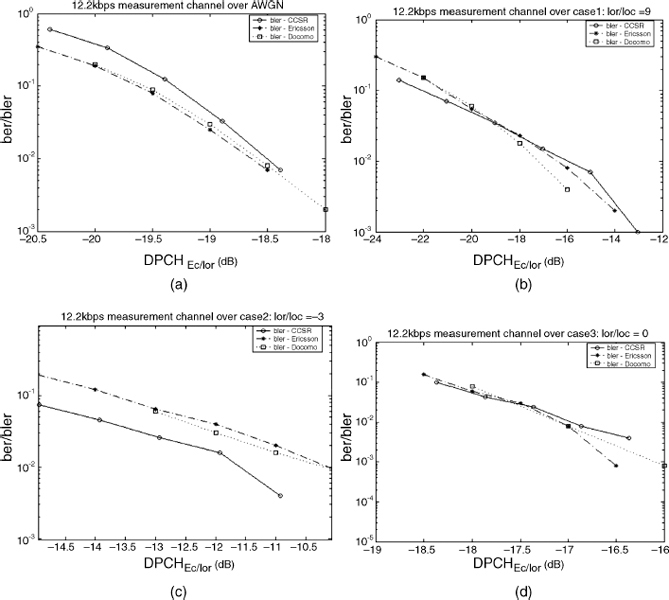
Figure 8.42 Comparison of reference performance for convolutional code use: (a) 12.2 kbps measurement channel over AWGN channel; (b) 12.2 kbps measurement channel over case 1 environment; (c) 12.2 kbps measurement channel over case 2 environment; (d) 12.2 kbps measurement channel over case 3 environment

8.3.3.4 UMTS DL Model Verification for Turbo Code Use

[30] also presents the upper bounds for performance of turbo codes under different propagation conditions. The results generated with the CCSR model at a BLER of 10% and 1% were compared to the above reference figures, as listed in Table 8.23 for the 64 kbps test channel and in Table 8.24 for the 144 kbps test channel.

The results listed in the tables clearly show that under the propagation conditions described in [30], the performance of the CCSR model at a resulting BLER of 10% and 1% is within the required maximum limits. As for convolutional codes, performance for turbo codes are evaluated and compared to performance figures obtained by Ericsson [28] and NTT DoCoMo [29]. The performance traces under different conditions are shown in Figure 8.43 for 64 kbps and in Figure 8.44 for 144 kbps. Dashed-dotted lines denote the results of Ericsson, while dashed lines with star marks show the results of NTT DoCoMo.

Table 8.23 Performance validation for 64 kbps channel

The result for case 1 is very close to the results given in the above references. The result over AWGN channel shows closer performance to Ericsson figures. As with the convolutional code, the CCSR model outperforms the other two models in the operation over case 2 propagation environment. However, for the 144 kbps channel over case 3, the CCSR model results do not closely follow the reference traces. Moreover, even the reference traces do not show close performance in this environment. There are several reasons for this behavior. First, case 3 resembles a typical outdoor vehicular environment. Mobile speed is set to 120 kmph in this condition. Therefore the effect of time-varying multipath channel conditions and intercell interference are more evident in this condition, resulting in a variation in performance. Second, the implementation of the intercell interference could be different in each model. In the CCSR model, intercell interference is evaluated mathematically and is mapped on to the variance of the Gaussian noise source. Third, the decoding algorithm used for turbo iterative decoding in the CCSR model is the LogMap algorithm, while the reference models use the MaxLogMap algorithm. Even though these two algorithms show similar performance for AWGN channels, when applied over multipath propagation conditions their performance depends on other conditions, such as the length of the turbo-internal interleaver, input block length, and input signal amplitude [42].

Table 8.24 Performance validation for 144 kbps channel

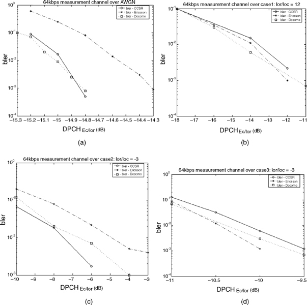
Figure 8.43 Comparison of reference performances for 64 kbps channel: (a) 64 kbps measurement channel over AWGN environment; (b) 64 kbps measurement channel over case 1 environment; (c) 64 kbps measurement channel over case 2 environment; (d) 64 kbps measurement channel over case 3 environment

8.3.4 UMTS Physical Link Layer Simulator

From a user point of view, services are considered end-to-end; that means from one terminal equipment to another terminal equipment. An end-to-end service may have a certain quality of service, which is provided for the user by the different networks. In UMTS, it is the UMTS bearer service that provides the requested QoS, through the use of different QoS classes, as defined in [45]. At the physical layer, these QoS attributes are assigned a radio access bearer (RAB) with specific physical-layer parameters in order to guarantee quality of service over the air interface. RABs are normally accompanied by signaling radio bearers (SRBs). Typical parameter sets for reference RABs, signaling RBs, and important combinations of the two (downlink, FDD) are presented in [37]. In the simulation, 3.4 kbps SRB, which is specified in [37], is used for the dedicated control channel (DCCH). Transport channel parameters for the 3.4 kbps SRB are summarized in Table 8.25.

Figure 8.44 Comparison of reference performances for 144 kbps channel: (a) 144 kbps measurement channel over AWGN environment; (b) 144 kbps measurement channel over case 1 environment; (c) 144 kbps measurement channel over case 2 environment; (d) 144 kbps measurement channel over case 3 environment

Careful examination of parameter sets for RABs and SRBs, which are specified in [37], shows that the minimum possible rate-matching ratios for RABs and SRBs vary with the physical-layer spreading factor being used. This is because when a higher spreading factor is used it adds transmission channel protection to the transmitted data in addition to the channel protection provided by the channel coding. Therefore, the channel bit error rate reduces with increase in spreading factor, and it is possible to allow higher puncturing in these scenarios without loss of performance. Table 8.26 shows the variation of calculated minimum rate-matching ratios (maximum puncturing ratio) with a spreading factor for FDD downlink control channels.

Table 8.25 Transport channel parameter for 3.4 kbps signaling radio bearer [37]. Reproduced, with permission, from “3rd Generation Partnership Project; technical specification group terminals; common test environments for user equipment (UE) conformance testing (release 4)”, 3GPP TS 34.108 V4.7.0 (2003–06). ©2003 3GPP. ©1998 3GPP. Reproduced by permission of © European Telecommunications Standards Institute 2008. Further use, modification, redistribution is strictly prohibited. ETSI standards are available from http://pda.etsi.org/pda/

In the simulation, rate-matching attributes for an SRB are set according to the minimum rate-matching ratios shown in Table 8.26 for different physical channels. The actual information data rate is a function of spreading factor, rate-matching ratio, type of channel coding, channel coding rate, number of CRC bits, and transport block size. Table 8.27 is a list of all the parameters that are user-definable, either by modifying the parameters of hierarchical models, by changing the building blocks that constitute the model, or by using different schematics.

8.3.4.1 BLER/BER Performance of Simulator

Simulations were carried out for different radio bearer configuration settings. For higher spreading factor realizations, the simulation period was set to 60 s duration. However, for spreading factor 8, the simulation period was limited to 30 s. This is to compensate for the higher processing time requirement seen at high data rates. 3000–6000 radio frames (10 ms) accommodate about 15 000–20 000 RLC blocks in a generated bit error sequence, and that is sufficiently long enough to obtain a meaningful BLER average. Furthermore, experimental results show that the selected simulation duration is sufficient to capture the bursty nature of the wireless channel and its effect on the perceptual quality of received video.

Table 8.26 Minimum rate matching ratios for SRB

SF	Minimum rate matching ratio
128	0.690
64	0.73
32	0.99
16–4	1.0

Table 8.27 UTRAN simulator parameters

Parameters	Settings
CRC attachment	24, 16, 12, 8 or 0
Channel coding scheme supported	No coding, 1/2 rate convolutional coding, 1/3 rate convolutional coding, 1/3 rate turbo coding
Interleaving	1st interleaving: block interleaver with interframe permutation 2nd interleaving: block interleaver with inter-columns permutation (Permutation patterns are specified in [38])
Rate matching	The algorithm (for convolutional rate matching) as specified in 3GPP TS 25.212. Rate matching ratio (repeat or puncturing ratio) is user-definable
TrCH multiplexing	Experiments were conducted for two transport channels
Transport format detection	TFCI-based detection
Spreading factor	512, 256, 128, 64, 32, 16, 8, 4
Transmission time interval	10 ms, 20 ms, 40 ms, 80 ms
Pilot bit patterns	As specified in 3GPP TS 25.211
Interference/noise characteristics	User-defined values are converted to the variance of AWGN source at receiver
Fading characteristics	Rayleigh fading mobile channel impulse response is updated 100 times for every coherence time interval
Multipath characteristics	Vehicular, pedestrian
Mobile terminal velocity	User-definable. Constant for the simulation run
Chip rate	3.84 Mcps
Carrier frequency	2000 MHz
Antenna characteristics	0 dB gain for both transmitter and receiver antenna
Receiver characteristics	Rake receiver with maximum ratio combining, equal gain combining, or selective combining. Number of rake fingers is user-definable
Transmission diversity characteristic	Closed-loop fast power control [46]
Channel decoding	Soft-decision Viterbi convolutional decoder Standard LogMap turbo decoder Number of turbo iterations is user-definable
Performance measures	Bit error patterns and block error patterns
Simulation length	3000–6000 radio frames, equivalent to 30–60 s duration

Effect of Spreading Factor

For the purpose of a performance comparison of the effect of spreading-factor variation, experiments were conducted for various spreading-factor allocations. The other physical channel parameters are set to their nominal values, which are shown in Table 8.28. The calculated possible information data rates are based on the specified SRBs for a given composite transport channel (consisting of one signaling channel and one dedicated data channel) for FDD downlink channels and are presented in Table 8.29. Table 8.29 also lists the RLC payload setting used in different bearer configurations.

Table 8.28 Nominal parameter settings

Spreading Factor	32
Transmission Time Interval	20 ms
CRC Attachment	16 bits
Channel Coding	1/2 CC, 1/3 CC, 1/3 TC
Mobile Speed	3 kmph, 50 kmph
Rate Matching Ratio	1.0
Operating Environment	Vehicular A, pedestrian B

Table 8.29 Channel throughput characteristics

Figure 8.45 shows the BER performance for the transmission of uncoded data (raw BER/channel BER) over the vehicular A propagation environment. It clearly illustrates the error-flow characteristics experienced due to the intersymbol interference in multipath channels. The effect of intersymbol interference increases with a reduction in spreading factor. However, the error-flow characteristic is not very pronounced in terms of coded BER performance, except for very low spreading factor allocations (see Figure 8.46). This is due to the effect of the channel coding algorithm, which tends to correct most of the errors if the channel bit error ratio is lower than 10⁻².

Figure 8.46(a) shows the performance of convolutional code, while the performance of turbo code is shown in Figure 8.46(b). The effect of spreading factor variation on the performance of turbo codes is similar to that of convolutional codes. However, the performance for spreading factor 8 is closer to that of other spreading factors than to the convolutional coding case. This is mainly due to the behavior of turbo codes. It is known that the higher the input block size of the turbo code, the better the performance. A high-bit-rate (with low spreading factor) service can accumulate more bits in a TTI than a low-bit-rate service. The better performance of the turbo code seen with large input block sizes compensates for the reduced robustness against interference provided by low spreading factor realizations. In Figure 8.46(a) and (b), the performance for 128 spreading factor is worse than that for 16 and 32 spreading factors. A possible reason is the poor performance of the interleavers (the first interleaver in convolutional coding and the first and turbo internal interleaver in turbo coding) in the presence of smaller input block sizes.

Figure 8.45 Performance of uncoded channel over vehicular A environment

Effect of Channel Coding

Figure 8.47 illustrates the effect of channel coding schemes on the block error ratio and bit error ratio performances. The vehicular A channel environment is considered the test environment, while the spreading factor is set to 32. As expected, turbo coding shows better performance than the other channel coding schemes, while the 1/3 rate convolutional code outperforms the 1/2 rate convolution code. It must be emphasized that the plots shown are the BLER/BER performances vs E_b/N_o. If the BLER/BER performances are viewed vs transmitted power, significant improvements will be visible for the 1/3 rate coding scheme compared to the 1/2 rate coding scheme. This is because the transmit power is directly proportional to the source bit rate. As 1/2 rate coding supports higher source rates, the corresponding curve will be shifted more to the right than others. Furthermore, the convolutional code and the turbo code show closer BLER performance (shown in Figure 8.47(b)) than the BER performance shown in Figure 8.47(a). This is due to the properties of the implemented LogMap algorithm at the turbo decoder, which is optimized to minimize the number of bit errors rather than the block error ratio [42].

Figure 8.46 Spreading factor effect for vehicular A environment: (a) 1/3 rate convolutional code; (b) 1/3 rate turbo code

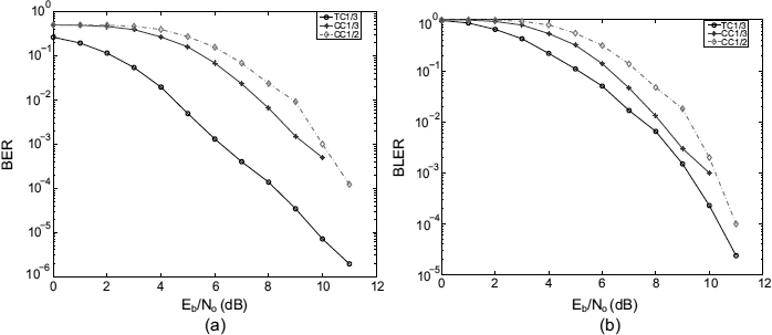
Figure 8.47 Effect of channel coding scheme: (a) BER; (b) BLER performance

Effect of Channel Environment

Experiments were conducted to investigate the BLER performance for the pedestrian B channel environment. The mobile speed is set to 3 kmph. Results for 1/3 rate convolutional code with different spreading factors are shown in Figure 8.48. As is evident from the figure, the resulting performance over the pedestrian B channel is much lower than that over the vehicular A channel environment when operating without fast power control. This is due to the slow channel variation associated with low mobile speeds. A larger number of consecutive information blocks can experience a long weaker channel condition during the transmission. This reduces the performance of block-based de-interleaving and channel decoding algorithms, resulting in a high block error ratio. On the other hand, a faster Doppler effect results in alternating weak and strong channel conditions of short durations at high vehicular speeds. This effect behaves as a time-domain transmit diversity technique and enhances the performance of block-based interleaving and channel coding algorithms.

Figure 8.48 1/3 rate convolutional coding performance for the pedestrian B environment

8.3.4.2 E_b/N_o to E_b/I_o and C/I Conversion

The BER performance of UMTS-FDD systems depends on many factors, such as mean bit energy of the useful signal, thermal noise, and interference. Interference can be divided into three main parts, as intersymbol interference, intra-cell interference, and inter-cell interference. Due to the multiple receptions, the signal is received with significant delay spread in a multipath propagation environment. This causes the intersymbol interference. Orthogonal codes are used to separate users in the downlink. Without any multipath propagation, these codes can be considered as perfectly orthogonal to each other. However, in a multipath propagation environment, orthogonality among spreading codes deviates from perfection, due to the presence of delay spread of the received signal. Therefore, the mobile terminal sees part of the signal, which is transmitted to other users, as interference power, and it is labeled intra-cell interference. The interference power seen among users in neighboring cells is quantified as the inter-cell interference.

BER performance is commonly written as a function of the global E_b/η, where the definition is given as:

where E_b is the received energy per bit of the useful signal, N_o is the power density representing the system-generated thermal noise, η is the global noise power spectrum density, χ is the intercell interference power spectral density, ρ is the orthogonality factor (OF), I_o is the intra-cell interference power spectral density, and η_ISI is the power spectral density of the intersymbol interference of the received signal.

These factors depend on:

• The operating environment.
• The number of active users per cell.
• The used spreading factors in the code tree.
• The cell site configurations.
• Presence of the diversity techniques.
• The mobile user locations.
• The type of radio bearer.
• The voice activity factor.

The loss of orthogonality between simultaneously-transmitted signals on a WCDMA downlink is quantified by the OF. The lower the value of the OF, the smaller the interference; an OF of 1 corresponds to the perfect orthogonal case, while an OF near 0 indicates considerable downlink interference. The introduction of the orthogonality factor in modeling intra-cell interference allows the employment of the Gaussian hypothesis. It is employed where the equivalent Gaussian noise with power spectral density is equal to (1 − ρ) times the received intra-cell interference power, and is simply added at the receiver input. The statistics of the OF are normally derived from measurement data gathered through extensive field trial campaigns. In the designed UTRA downlink simulator, the OFs, which are derived based on the gathered channel data and are presented in [47], are used to simulate the intra-cell interference power.

The inter-cell interference can also be modeled with the Gaussian hypothesis. The inter-cell interference power spectral density and the intra-cell interference power spectral density can be explicitly obtained through system-level simulations or analytical calculations based on simplifying assumptions and cell configuration [31]. However, intersymbol interference can only be obtained by chip-level simulation and does not depend on other factors, apart from used spreading factor, propagation condition, and mobile speed. Therefore, it is sufficient to obtain the E_b/η performance for one single connection (χ = 0, I_o = 0) of each of all the possible bit rates or spreading factors by chip-level simulation. Then the E_b/I_o performances can easily be derived from E_b/η using Equation (8.14). is assumed, and the intersymbol interference is implicit in the simulation.

Equation (8.15) shows the relationship between average energy per bit and average received signal power, S.

where R denotes data bit rate.

Therefore:

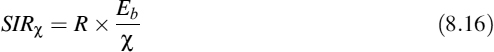
Table 8.30 Orthogonality factor variation for different cellular environments [47]

[T]where SIR_χ, SIR_I, and SIR_Total denote signal-to-inter-cell interference ratio, signal-to-intra-cell ratio, and signal-to-interference ratio respectively.

Assume N_o = 0.0002, χ = 0.005, and vehicular A propagation environment. From Table 8.30, the orthogonality factor is 0.514. The E_b/I_o for E_b/η values shown in Figure 8.46(a) are calculated from Equation (8.14) and are shown in Figure 8.49.

8.3.5 Performance Enhancement Techniques

8.3.5.1 Fast Power Control for Downlink

As can be seen in Figure 8.48, data transmission over the pedestrian B slow-speed propagation environment shows worse performance than over the high-speed propagation environment. This is mainly because the error-correcting methods are based on the interleaving and block-based methods, which do not work effectively in the presence of long-duration weak channel conditions caused by Rayleigh fading at low mobile speeds. This condition (weak long radio link) can be improved by the application of a fast power control algorithm. A closed-loop fast power control algorithm has been designed and is incorporated in the simulator. The implementation and the resulting performance improvement are described below.

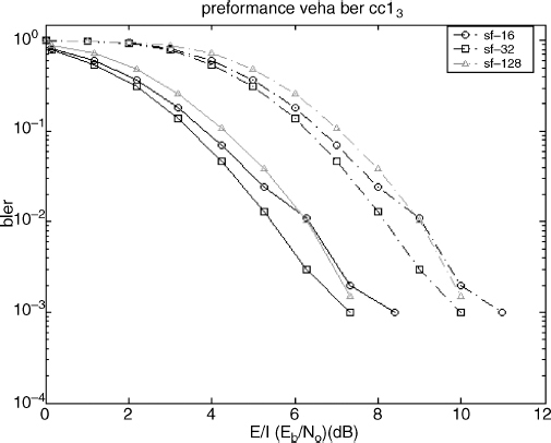
Figure 8.49 BLER performance: solid line shows BLER vs. E_b/N_o; dashed line shows BLER vs. E_b/η

Figure 8.50 Fast power control for UTRA-FDD downlink

8.3.5.2 Algorithm Implementation

A block diagram representation of the implemented power control algorithm is depicted in Figure 8.50. According to the measured received pilot power at the receiver, the UE generates appropriate transport power control (TPC) commands (whether to adjust transmit power up or down) to control the network transmit power and sends them in the TPC field of the uplink dedicated physical control channel (DPCCH). The TPC command decision is made by comparing the average received pilot power (averaged over an integer number of slots to mitigate the effects of varying interference and noise) to the pilot power threshold, which is predefined by the UTRAN based on the outer-loop power control [48]. Upon receiving the TPC commands, UTRAN adjusts its downlink DPCCH/DPDCH power according to Equation (8.19).

where P(k) denotes the downlink transmit power in the kth slot, and Δ_TPC is the power control step size. ± is decided from the uplink TPC command. This algorithm is executed at a rate of 1500 times per second for each mobile connection. Settings used in the implementation are listed in Table 8.31.

Note: the aggregated power control step is defined as the required total changes in a code channel in response to ten multiple consecutive power control commands.

Table 8.31 Power control parameter settings [48]

Power Control Step Size	0.5 ± 0.25 dB
Aggregated Power Control Step Change	4–6 dB
Power Averaging Window Size, n	4
Feedback Delay	3 slots
Algorithm Execution Frequency	1.5 kHz

Figure 8.51 Characteristic of the fast power control algorithm

The control algorithm adjusts the power of the DPCCH and DPDCH; however, the relative power difference between the two is not changed.

Figure 8.51 shows how a downlink closed-loop power control algorithm works on a fading channel at low vehicular speed. Node B transmit power varies inversely proportional to the received pilot power. This closely resembles the time-varying channel at low mobile speeds. Transmit power cut-off values are defined by the maximum and minimum power limits set by node B. Receive power at the receiver shows very little residual fading.

Figure 8.52 illustrates the performance of the power control algorithm for data transmission over the vehicular A propagation environment with a spreading factor 16 and 1/3 rate convolutional coding. The experiment was carried out at three different mobile speeds settings, namely 3, 50 and 120 kmph. The performance improvement by power control is evident at low speed, while at high mobile speed the improvement is largely insignificant. This is because a transmission diversity gain is provided by the highly time-varying channel at high mobile speed.

8.3.6 UMTS Radio Interface Data Flow Model

The designed physical link layer simulator alone provides a necessary experimental platform to examine the effects of the radio link upon the data transmitted through the physical channel. However, in order to investigate the effect of channel bit errors upon the end-application, the application performance must be validated in an environment as close as possible to that of the real world. Therefore, not only the effect of the physical link layer but also the effect of UMTS protocol layer operation on multimedia performance should be investigated. A UMTS data flow model was designed in Microsoft Visual C++ to emulate the protocol layer behavior. The design criteria follow a modular design strategy. Each of the protocol layers was implemented separately and protocol interaction is performed through the specified interfaces. This allows individual protocol-layer optimization, or improvement and testing of novel performance-enhancement algorithms in the presence of a complete system. Here, only the protocol-layer effect on multimedia performance is considered. The protocol layers implemented include the application layer, transport layer, PDCP layer, RLC/MAC layer, and layer 1. The block diagram of the data flow model is shown in Figure 8.53. The effect of protocol headers on application performance was emulated by allocating dummy headers.

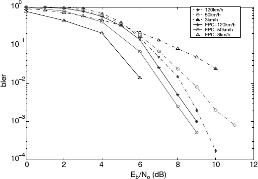
Figure 8.52 Fast power control algorithm performance

The application consists of a full error-resilience-enabled MPEG-4 video source. In addition to the employed error-resilience techniques, the TM5 rate-control algorithm is used in order to achieve a smoother output bit rate. An adaptive intra refresh algorithm is also implemented to stop temporal error propagation and to achieve a smoother output bit rate. The output source bit rate is set according to the guaranteed bit rate, which is a user-defined QoS parameter. For packet-switched connections, encoded video frames are forwarded to the transport layer at regular intervals, as defined by the video frame rate. Each video frame is encapsulated into an independent RTP/UDP/IP packet [22] for forwarding down to the PDCP layer. The PDCP exists mainly to adapt transport-layer packet to the radio environment by compressing headers with negotiable algorithms [49]. The current version of the data flow model implements the resulting compressed header sizes, but not the actual header-compression algorithms. More extensive and detailed examination of different header-compression algorithms and their effects on multimedia performance can be found in [50]. For circuit-switched connections, the output from the video encoder is directly forwarded to the RLC/MAC layer.

At the RLC layer, forwarded information data is further segmented into RLC blocks. The size of an RLC block is defined by the transport block (TB) size, which is an implementation-dependent parameter. Optimal setting of TB size should include many factors, such as application type, source traffic statistics, allowable frame delay jitter, and RLC buffer size. RLC block header size depends on the selected RLC mode for the transmission. Transparent mode adds no header as it transmits higher-layer payload units transparently. Unacknowledge mode and acknowledgement mode add 8 bit and 16 bit headers to each RLC block, respectively [34]. Apart from the segmentation and addition of a header field, other RLC layer functions such as error detection and retransmission of erroneous data are not implemented in the current version of the model as the main use of the model is to investigate the performance of conversational-type multimedia applications. The MAC layer can be either dedicated or shared. A dedicated mode is responsible for handling dedicated channels allocated to a UE in connected mode, while shared mode takes responsibility for handling shared channels. If channel multiplexing is performed at the MAC layer then a 4 bit MAC header is added to each RLC block [35].

Figure 8.53 UTRAN data flow model

Layer 1 attaches a CRC to forwarded RLC/MAC blocks. According to the specified TTI length, higher-layer blocks are combined to form the TTI blocks and store them in a buffer for further processing before transmitting over the air interface. The number of higher-layer PDUs to be encapsulated within the TTI block depends on the selected channel coding scheme, the spreading factor, and the rate-matching ratio. In a practical system, the selection of channel coding scheme, TTI length, and CRC size is normally performed by the radio resource management algorithm according to the end user quality requirement, application type, operating environment, system load, and so on. For experimental sake, these parameters are to be user-definable in the designed data flow model. An error-prone radio channel environment is emulated by applying generated bit errors from the physical link layer simulator to the information data at layer 1.

The receiver side is emulated by reversing the described processing. Layer 1 segments the TTI blocks received over the simulated air interface into RLC/MAC blocks. After detaching CRC bits, RLC/MAC blocks are passed on to the RLC/MAC layer. At the RLC/MAC layer the received data is reassembled into PDCP data units for packet-switched connections. If IP/UDP/RTP headers are found to be corrupted, data encapsulated within the packet is dropped at the network layer. Finally, the received source data is displayed using an MPEG-4 decoder.

This layered implementation of the UMTS protocol architecture allows the investigation of the effects of physical layer-generated bit errors upon different fields of the payload data units at each protocol layer. In other words, the data flow model can be used to map channel errors on to different PDU fields and to optimize protocol performance for the given application.

8.3.7 Real-time UTRAN Emulator

The above-described UMTS data flow model is integrated with the physical link layer model to form the UTRAN emulator. The emulator software suite provides a graphical user interface for connection setup, radio bearer configuration, and performance monitoring. The emulator model considers the emulated system to be a black box, whose input–output behavior intends to reproduce the real system without requiring knowledge of the internal structure and processes. It has also been designed for accurate operation in real time with moderate implementation complexity. The emulator was implemented in Visual C++, as it provides a comprehensive graphical user interface design environment.

Figure 8.54 depicts the block diagram of the designed emulator architecture. It consists of three main parts, namely content server, UMTS emulator, and mobile client. An “MPEG-4 file transmitter” is used as the content server. It selects the corresponding video sequence, which is encoded according to the requested source bit rate, frame rate, and other error-resilience parameters, and transmits the video to the UMTS radio link emulator. At the emulator the received source data passes through the UMTS data flow model and the simulated physical link layer, and is finally transmitted to the mobile client for display. Here, a PC-based MPEG-4 decoder is used to emulate the display capabilities of the mobile terminal.

The UMTS configuration options dialog box (Figure 8.55) is designed for interactive radio bearer configuration for a particular connection. The QoS parameter page shows the user-requested quality of service parameters, such as type of service, traffic class, data rates, residual bit error ratio, and transfer delay. In addition, operator control parameters, connection type, PDCP connection type, and the number of multiplexed transport channels are shown.

The transport channel parameter page for the data channel shows the transport channel-related network parameter settings (Figure 8.56). Logical channel type, RLC mode, MAC channel type, MAC multiplexing, layer 1 parameters, TTI, channel coding scheme, and CRC are user-definable emulator parameters, while TB size and rate matching ratio are calculated and displayed from the other input parameter values. If the number of multiplexed transport channels is set to 1 then the transport channel parameter page for the control channel is disabled. Otherwise it shows the transport channel parameters that are related to the control channel.

The appropriate spreading factor for transmission is calculated based on the requested QoS parameters and is displayed on the physical/radio channel parameter page (Figure 8.57). Radio channel-related settings (carrier frequency, channel environment, mobile speed) and receiver characteristics (number of rake fingers, rake combining, diversity techniques, power control) are selected on the physical/radio parameter page.

Figure 8.54 UMTS emulator architecture

Figure 8.58 illustrates the user interfaces of the designed emulator. In addition to the radio bearer configuration parameter pages described so far, the emulator also displays the instantaneous performance in terms of E_b/N_o, E_b/I_o, C/I, and BER. Furthermore, it allows interactive manipulation of the number of users in the cell (hence co-channel interference), and monitoring of the video performance in a more realistic operating environment.

8.3.8 Conclusion

The design and evaluation of a UMTS-FDD simulator for the forward link has been described. The CCSR model gives performances that satisfy the requirements shown in 3GPP performance figures. Furthermore, the performance of the CCSR model closely follows the performance traces published by different terminal manufactures on most test configurations. However, some performance variation was visible for operation over the case 2 propagation environment and 144 kbps reference channel over the case 3 test environment. As mentioned earlier, there are several things that could contribute to this. The most likely is the different implementation strategies followed in the receiver design and in channel decoding. Another possible contributor is the different simulation techniques used for propagation modeling and interference modeling. The differences seen in the performance of turbo codes are greater than in the performance of convolutional codes, where the coding/decoding technology is fairly stable and consolidated. In addition, the performance of the LogMap algorithm implementation (provided in the SPW package) is highly sensitive to the amplitude of the decoder input signal. The input amplitude setting was based on the conducted experimental results and may cause slight performance degradation.

Figure 8.55 QoS parameter option page

Figure 8.56 Transport channel parameter option page

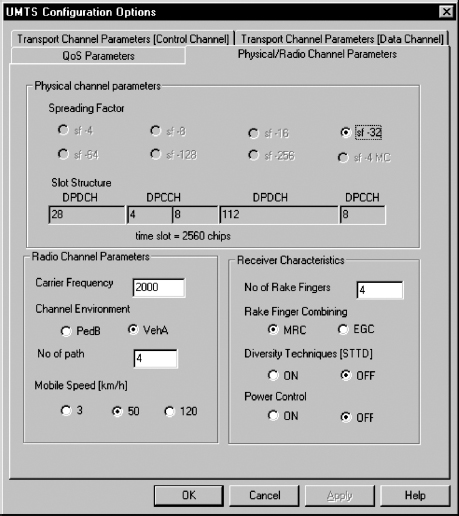
Figure 8.57 Physical/radio channel parameter option page

Even though the CCSR model matches the reference performance traces, or comes very close to them under the particular bearer configurations tested, the bit error sequences generated by the CCSR model should be considered, to a certain extent, as worst-case performance figures. The designed quasi-ideal rake receiver employs non-ideal channel estimation based on weighted multislot averaging (WMSA) techniques. The settings of the WSMA filter parameters might not be considered optimal in varying simulation environments. Also, the employment of advanced power control techniques can result in improved performance over the less complex fast power control algorithm implemented. In fact, the CCSR model shows about 3 dB performance loss over the results published by Olmos [51] using a non-ideal rake receiver and fast power control. The intention of the UMTS physical layer simulation model was to facilitate investigation of multimedia performance over the UMTS air interface. Although the performance test results were presented as block error ratio values, the output of the physical link simulator produces bit error sequences to characterize the actual physical link layer. After integrating with the UMTS protocol data flow model, the physical link layer-generated bit error patterns can be used in audiovisual transmission experiments. In addition to the high degree of correlation shown between the performance of the CCSR model and the quoted reference figures, generated bit error patterns are suitable for employment in a radio bearer optimization for multimedia communication, as they exhibit relative differences between various network parameter and interference settings despite the type of receiver architecture implemented.

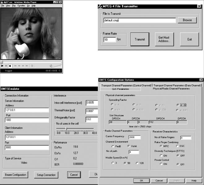
Figure 8.58 Real-time UTRAN emulator