2.3 Fundamentals of Video Compression

This section describes how spatial redundancy and temporal redundancy can be removed from a video signal. It also describes how a typical video codec combines the two techniques to achieve compression.

2.3.1 Video Signal Representation and Picture Structure

Video coding is usually performed with YUV 4:2:0 format video as an input. This format represents video using one luminance plane (Y) and two chrominance planes (Cb and Cr). The luminance plane represents black and white information, while the chrominance planes contain all of the color data. Because luminance data is perceptually more important than the chrominance data, the resolution of the chrominance planes is half that of the luminance in both dimensions. Thus, each chrominance plane contains a quarter of the pixels contained in the luminance plane. Downsampling the color information means that less information needs to be compressed, but it does not result in a significant degradation in quality.

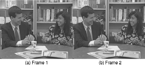
Figure 2.2 Temporal redundancy occurs when there is a large amount of similarity between video frames

Figure 2.3 Most video codecs break up a video frame into a number of smaller units for coding

Most video coding standards split each video frame into macroblocks (MB), which are 16 × 16 pixels in size. For the YUV 4:2:0 format, each MB contains four 8 × 8 luminance blocks and two 8 × 8 chrominance blocks, as shown in Figure 2.3. The two chrominance blocks contain information from the Cr and Cb planes respectively. Video codecs code each video frame, starting with the MB in the top left-hand corner. The codec then proceeds horizontally along each row, from left to right.

MBs can be grouped. Groups of MBs are known by different names in different standards. For example:

• Group of Blocks (GOB): H.263 [1–3]
• Video packet: MPEG-4 Version 1 and 2 [4–6]
• Slice: MPEG-2 [7] and H.264 [8–10]

The grouping is usually performed to make the video bitstream more robust to packet losses in communications channels. Section 2.4.8 includes a description of how video slices can be used in error-resilient video coding.

2.3.2 Removing Spatial Redundancy

Removal of spatial redundancy can be achieved by taking into account:

• The characteristics of the human vision system: human vision is more sensitive to low-frequency image data than high-frequency data. In addition, luminance information is more important than chrominance information.
• Common features of image/video signals: Figure 2.4 shows an image that has been high-pass and low-pass filtered. It is clear from the images that the low-pass-filtered version contains more energy and more useful information than the high-pass-filtered one.

Figure 2.4 ‘Lena’ image subjected to a high-pass and a low-pass filter

These factors suggest that it is advantageous to consider image/video compression in the frequency domain. Therefore, a transform is needed to convert the original image/video signal into frequency coefficients. The DCT is the most widely used transform in lossy image and video compression. It permits the removal of spatial redundancy by compacting most of the energy of the block into a few coefficients.

Each 8 × 8 pixel block is put through the discrete cosine transform (DCT):

where , N is the block size (N = 8),1 otherwise s(n₁, n₂) is an original image 8 × 8 block, and S(k₁, k₂) is the 8 × 8 transformed block.

Figure 2.5 Transform-based compression (a) Original image block (b) DCT transformed block

An example of the DCT in action is shown below, and illustrated in Figure 2.5. An input block, s(n₁, n₂), is first taken from an image:

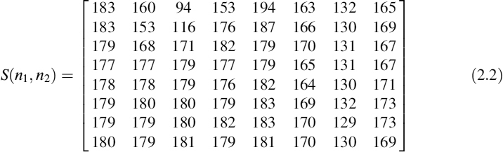
It is then put though the DCT, and is rounded to the nearest integer:

The coefficients in the transformed block represent the energy contained in the block at different frequencies. The lowest frequencies, starting with the DC coefficient, are contained in the top-left corner, while the highest frequencies are contained in the bottom-right, as shown in Figure 2.5.

Note that many of the high-frequency coefficients are much smaller than the low-frequency coefficients. Most of the energy in the block is now contained in a few low-frequency coefficients. This is important, as the human eye is most sensitive to low-frequency data.

It should be noted that in most video codec implementations the 2D DCT calculation is replaced by 1D DCT calculations, which are performed on each row and column of the 8 × 8 block:

for u = 0,1,2 …, N − 1. The value of α(u) is defined as:

The 1D DCT is used as it is easier to optimize in terms of computational complexity.

Next, quantization is performed by dividing the transformed DCT block by a quantization matrix. The standard quantization matrices used in the JPEG codec are shown below:

where Q_Y is the matrix for luminance (Y plane) and Q_UV is the matrix for chrominance (U and V planes). The matrix values are set using psycho-visual measurements. Different matrices are used for luminance and chrominance because of the differing perceptual importance of the planes.

The quantization matrices determine the output picture quality and output file size. Scaling the matrices by a value greater than 1 increases the coarseness of the quantization, reducing quality. However, such scaling also reduces the number of nonzero coefficients and the size of the nonzero coefficients, which reduces the number of bits needed to code the video.

2.3.2.1 H.263 Quantization Example

Take the DCT matrix from above:

and divide it by the luminance quantization matrix:

The combination of the DCT and quantization has clearly reduced the number of nonzero coefficients.

The next stage in the encoding process is to zigzag scan the DCT matrix coefficients into a new 1D coefficient matrix, as shown in Figure 2.6. Using the above example, the result is:

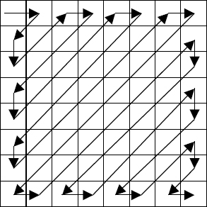
Figure 2.6 Zigzag scanning of DCT coefficients

Table 2.1 Run-level coding

where the EOB symbol indicates the end of the block (i.e. all following coefficients are zero). Note that the number of coefficients to be encoded has been reduced from 64 to 28 (29 including the EOB).

The data is further reorganized, with the DC component (the top-left in the DCT matrix) being treated differently from the AC coefficients.

DPCM (Differential Pulse Code Modulation) is used on DC coefficients in the H.263 standard [1]. This method of coding generally creates a prediction for the current block's value first, and then transmits the error between the predicted value and the actual value. Thus, the reconstructed intensity for the DC at the decoder, s(n₁, n₂), is:

where and e(n₁, n₂) are respectively the predicted intensity and the error.

For JPEG, the predicted DC coefficient is the DC coefficient in the previous block. Thus, if the previous DC coefficient was 15, the coded value for the example given above will be:

AC coefficients are coded using run-level coding, where each nonzero coefficient is coded using a value for the intensity and a value giving the number of zero coefficients preceding the coefficient. With the above example, the coefficients are represented as shown in Table 2.1.

Variable-length coding techniques are used to encode the DC and AC coefficients. The coding scheme is arranged such that the most common values have the shortest codewords.

2.3.3 Removing Temporal Redundancy

Image coding attempts to remove spatial redundancy. Video coding features an additional redundancy type: temporal redundancy. This occurs because of strong similarities between successive frames. It would be inefficient to transmit a series of JPEG images. Therefore, video coding aims to transmit the differences between two successive frames, thus achieving even higher compression ratios than for image coding.

The simplest method of sending the difference between two frames would be to take the difference in pixel intensities. However, this is inefficient when the changes are simply a matter of objects moving around a scene (e.g. a car moving along a road). Here it would be better to describe the translational motion of the object. This is what most video codec standards attempt to do.

A number of different frame types are used in video coding. The two most important types are:

• Intra frames (called I frames in MPEG standards): these frames use similar compression methods to JPEG, and do not attempt to remove any temporal redundancy.
• Inter frames (called P frames in MPEG): these frames use the previous frame as a reference.

Intra frames are usually much larger than inter frames, due to the presence of temporal redundancy in them. However, inter frames rely on previous frames being successfully received to ensure correct reconstruction of the current frame. If a frame is dropped somewhere in the network then all subsequent inter frames will be incorrectly decoded. Intra frames can be sent periodically to correct this. Descriptions of other types of frame are given in Section 2.4.1.

Motion compensation is the technique used to remove much of the temporal redundancy in video coding. It is preceded by motion estimation.

2.3.3.1 Motion Estimation

Motion estimation (ME) attempts to estimate translational motion within a video scene. The output is a series of motion vectors (MVs). The aim is to form a prediction for the current frame based on the previous frame and the MVs.

The most straightforward and accurate method of determining MVs is to use block matching. This involves comparing pixels in a certain search window with those in the current frame, as shown in Figure 2.7. Typically, the Mean Square Error is employed, such that the MV can be found from:

where is the optimum MV, s(n₁, n₂, k) is the pixel intensity at the coordinate (n₁, n₂) in the kth frame, and β isa16 × 16 block.

Thus, for each MB in the current frame, the algorithm finds the MV that gives the minimum MSE compared to an MB in the previous frame.

Figure 2.7 ME is carried out by comparing an MB in the current frame with pixels in the reference frame within a preset search window

Although this technique identifies MVs with reasonable accuracy, the procedure requires many calculations for a whole frame. ME is often the most computationally intensive part of a codec implementation, and has prevented digital video encoders being incorporated into low-cost devices.

Researchers have examined a variety of methods for reducing the computational complexity of ME. However, they usually result in a tradeoff between complexity and accuracy of MV determination. Suboptimal MV selection means that the coding efficiency is reduced, and therefore leads to quality degradation, where a fixed bandwidth is specified.

2.3.3.2 Intra/Inter Mode Decision

Not all MBs should be coded as inter MBs, with motion vectors. For example, new objects may be introduced into a scene. In this situation the difference is so large that an intra MB should be encoded. Within an inter frame, MBs are coded as inter or intra MBs, often depending on the MSE value. If the MSE passes a certain threshold, the MB is coded as Intra, otherwise inter coding is performed. The MSE-based threshold algorithm is simple, but is suboptimal, and can only be used when a limited number of MB modes are available. More sophisticated MB mode-selection algorithms are discussed in Section 2.4.3.

2.3.3.3 Motion Compensation

The basic intention of motion compensation (MC) is to form as accurate a prediction as possible of the current frame from the previous frame. This is achieved using the MVs produced in the ME stage.

Each inter MB is coded by sending the MV value plus the prediction error. The prediction error is the difference between the motion-compensated prediction for that MB and the actual MB in the current frame. Thus, the transmitted error MB is:

The prediction error is generally smaller in magnitude than the original, meaning that less bits are required to code the error. Therefore, the compression efficiency is increased by using MC.

2.3.4 Basic Video Codec Structure

The video codec shown in Figure 2.8 demonstrates the basic operation of many video codecs. The major components are:

• Transform and Quantizer: perform operations similar to the transform and quantization process described in Section 2.3.2.
• Entropy Coder: takes the data for each frame and maps it to binary codewords. It outputs the final bitstream.
• Encoder Control: can change the MB mode and picture type. It can also vary the coarseness of the quantization and perform rate control. Its precise operation is not standardized.
• Feedback Loop: removes temporal redundancy by using ME and MC.

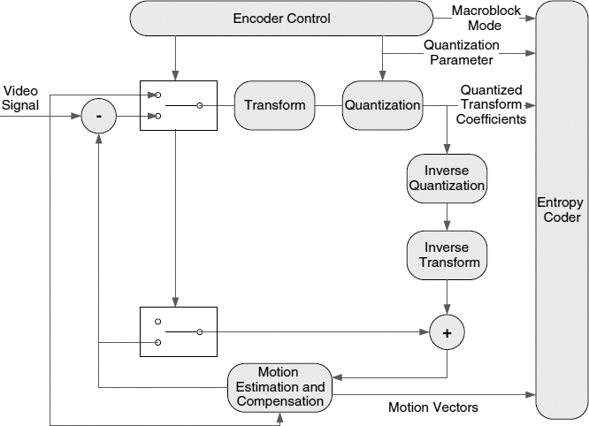
Figure 2.8 Basic video encoder block diagram