2.4 Advanced Video Compression Techniques

Section 2.3 discussed some of the basic video coding techniques that are common to most of the available video coding standards. This section examines some more advanced video coding techniques, which provide improved compression efficiency, additional functionality, and robustness to communication channel errors. Particular attention is paid to the H.264 video coding standard [8, 9], which is one of the most recently standardized codecs. Subsequent codecs, such as scalable H.264 and Multi-view Video Coding (MVC) [11], use the H.264 codec as a starting point. Note that scalability is discussed in Chapter 3.

2.4.1 Frame Types

Most modern video coding standards are able to code at least three different frame types:

• I frames (intra frames): these do not include any motion-compensated prediction from other frames. They are therefore coded completely independently of other frames. As they do not remove temporal redundancy they are usually much larger in size than other frame types. However, they are required to allow random access functionality, to prevent drift between the encoder and decoder picture buffers, and to limit the propagation of errors caused by packet loss (see Section 2.4.8).
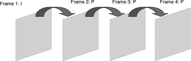
• P frames (inter frames): these include motion-compensated prediction, and therefore remove much of the temporal redundancy in the video signal. As shown in Figure 2.9, P frames generally use a motion-compensated version of the previous frame to predict the current frame. Note that P frames can include intra-coded MBs.

  

  Figure 2.9 P frames use a motion-compensated version of previous frames to form a prediction of the current frame

• B frames: the ‘B’ is used to indicate that bi-directional prediction can be used, as shown in Figure 2.10. A motion-compensated prediction for the current frame is formed using information from a previous frame, a future frame, or both. B frames can provide better compression efficiency than P frames. However, because future frames are referenced during encoding and decoding, they inherently incur some delay. Figure 2.11 shows that the frames must be encoded and transmitted in an order that is different from playback. This means that they are not useful in low-delay applications such as videoconferencing. They also require additional memory usage, as more reference frames must be stored.

H.264 supports a wider range of frames and MB slices. In fact, H.264 supports five types of such slice, which include I-type, P-type, and B-type slices. I-type (Intra) slices are the simplest, in which all MBs are coded without referring to other pictures within the video sequence. If previously-coded images are used to predict the current MB it is a called P-type (predictive) slice, and if both previous- and future-coded images are used then it is called a B-type (bi-predictive) slice.

Other slices supported by H.264 are the SP-type (Switching P) and the SI-type (Switching I), which are specially-coded slices that enable efficient switching between video streams and random access for video decoders [12]. A video decoder may use them to switch between one of several available encoded streams. For example, the same video material may be encoded at multiple bit rates for transmission across the Internet. A receiving terminal will attempt to decode the highest-bit-rate stream it can receive, but it may need to switch automatically to a lower-bit-rate stream if the data throughput drops.

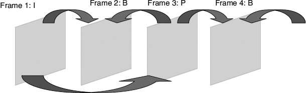
Figure 2.10 B frames use bi-directional prediction to obtain predictions of the current frame from past and future frames

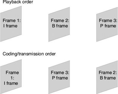
Figure 2.11 Use of B frames means that frames must be coded and decoded in an order that is different from that of playback

2.4.2 MC Accuracy

Providing more accurate MC can significantly reduce the magnitude of the prediction error, and therefore fewer bits need to be used to code the transform coefficients. More accuracy can be provided either by allowing finer motion vectors to be used, or by permitting more motion vectors to be used in an MB. The former allows the magnitude of the motion to be described more accurately, while the latter allows for complex motion or for situations where there are objects smaller than an MB.

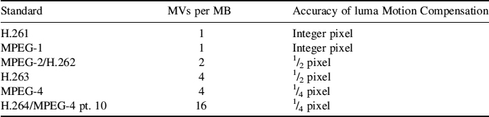
H.264 in particular supports a wider range of spatial accuracy than any of the existing coding standards, as shown in Table 2.2. Amongst earlier standards, only the latest version of MPEG-4 Part 2 (version 2) [5] can provide quarter-pixel accuracy, while others provide only half-pixel accuracy. H.264 also supports quarter-pixel accuracy.

For achieving quarter-pixel accuracy, the luminance prediction values at half-sample positions are obtained by applying a 6-tap filter to the nearest integer value samples [9]. The luminance prediction values at quarter-sample positions are then obtained by averaging samples at integer and half-sample positions.

An important point to note is that more accurate MC requires more bits to be used to specify motion vectors. However, more accurate MC should reduce the number of bits required to code the quantized transform coefficients. There is clearly a tradeoff between the number of bits added by the motion vectors and the number of bits saved by better MC. This tradeoff depends upon the source sequence characteristics and on the amount of quantization that is used. Methods of finding the best tradeoff are dealt with in Section 2.4.3.

Table 2.2 Comparison of the ME accuracies provided by different video codecs

2.4.3 MB Mode Selection

Most of the widely-used video coding standards allow MBs to be coded with a variety of modes. For example:

• MPEG-2: INTRA, SKIP, INTER-16 × 16, INTER-16 × 8.
• H.263/MPEG-4: INTRA, SKIP, INTER-16 × 16, INTER-8 × 8.
• H.264/AVC: INTRA-4 × 4, INTRA-16 × 16, SKIP, INTER-16 × 16, INTER-16 × 8, INTER-8 × 16, INTER-8 × 8; the 8 × 8 INTER blocks may then be partitioned into 4 × 4, 8 × 4, 4 × 8.

Selection of the best mode is an important part of optimizing the compression efficiency of an encoder implementation. Mode selection has been the subject of a significant amount of research. It is a problem that may be solved using optimization techniques such as Lagrangian Optimization and dynamic programming [13]. The approach currently taken in the H.264 reference software uses Lagrangian Optimization [14].

For mode selection, Lagrangian Optimization may be carried out by minimizing the following Lagrangian cost for each coding unit:

where R_REC(M, Q) is the rate from compressing the current coding unit with mode, M, and with quantizer value, Q. D_REC(M, Q) is the distortion obtained from compressing the current coding unit using mode, M, and quantizer, Q. The distortion can be found by taking the sum of squared differences:

where A is the MB, s is the original MB pixels, and s′ is the reconstructed MB pixels.

The remaining parameter, λ_MODE, can be determined experimentally, and has been found to be consistent for a variety of test sequences [15]. For H.263, the following curve fits the experimental results well:

where Q_H.263 is the quantization parameter.

For H.264, the following curve has been obtained:

where Q_H.264 is the quantization parameter for H.264.

For both H.263 and H.264, rate control can be performed by varying the quantization. Once rate control has been performed, the quantization parameter can be used to calculate λ, so that Lagrangian Optimization can be used to find the optimum mode. Results have shown that this kind of scheme can bring considerable benefits in terms of compression efficiency [14].

However, a major disadvantage of this type of optimization is that it involves considerable computational complexity. Many researchers have attempted to find lower-complexity solutions to this problem. Choi et al. describe one such scheme [16].

2.4.4 Integer Transform

Similar to earlier standards, H.264 also applies a transform to the prediction residual. However, it does not apply the conventional floating-point 8 × 8 DCT transform. Instead, a separable integer transform is applied to 4 × 4 blocks of the picture [17]. This transform eliminates any mismatches between encoder and decoder in the inverse transform due to precise integer specification. In addition, its small size helps in reducing blocking and ringing artifacts. For an MB coded in intra-16 × 16 mode, a similar 4 × 4 transform is performed for 4 × 4 DC coefficients of the luminance signal. The cascading of block transforms is equivalent to an extension of the length of the transform functions.

If X is the original image block then the 4 × 4 pixel DCT of X can be found:

The integer transform of H.264 is similar to the DCT, except that some of the coefficients are rounded and scaled, providing a new transform:

where E is a scaling factor. Note that the transform can be implemented without any multiplications, as it only requires additions and bit shifting.

Figure 2.12 Use of surrounding pixel values with intra prediction

2.4.5 Intra Prediction

In many video signals, adjacent MBs tend to have similar properties. These spatial redundancies can be reduced using Intra prediction of MBs. For a given MB, its predicted representation is calculated from already-encoded neighboring MBs. The difference between the predicted MB and the actual MB is transformed and quantized. The difference will usually be of smaller magnitude than the original block, and therefore will need fewer bits to code. In some previous standards, prediction was performed in the transform domain, while in H.264 it is now done in the spatial domain, by referring to neighboring samples [9].

H.264 provides two classes of intra coding, the INTRA-4 × 4 and INTRA-16 × 16, based on the size of sub-blocks over which prediction is estimated. When using the INTRA-4 × 4 mode, each 4 × 4 block of the luminance component utilizes one of nine available prediction options. Beside DC prediction (Mode 2), eight directional prediction modes are specified, which are labeled as 0, 1, 3, 4, 5, 6, 7, 8 in Figure 2.12. As shown in Figure 2.13, components from a to p are predicted from A to M components, and this prediction depends upon the selected mode.

INTRA-16 × 16 mode is more suitable for smooth image areas as it performs a uniform prediction for all of the luminance components of an MB. The chrominance samples of an MB are also predicted, using a similar prediction technique to that for a luminance component.

2.4.6 Deblocking Filters

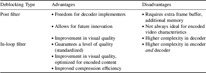
One particular characteristic of block-based coding is the appearance of block structures in decoded images. This feature is more prominent at low bit rates. Deblocking filters can be deployed to improve the perceived video quality. These filters can either be implemented inside the coding loop, or as a post-processing step at the decoder. Table 2.3 summarizes the advantages and disadvantages of each approach.

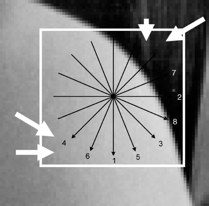
Figure 2.13 Intra prediction uses a number of different ‘directions’ to determine how to calculate the predicted intra block

An adaptive filter is applied to the horizontal and vertical edges of the MB within the prediction loop of H.264 [18]. The filter automatically varies its own strength, depending on the quantization parameter and the MB modes. This is to prevent filtering on high-quality video frames, where the filtering would degrade rather than improve quality.

The filtered MB is also used for motion-compensated prediction of further frames in the encoder, resulting in a smaller residual after prediction, and hence better compression efficiency.

Table 2.3 Comparison of the use of post-filter and in-loop-filter deblocking algorithms

2.4.7 Multiple Reference Frames and Hierarchical Coding

Long–term-memory motion-compensated prediction involves the possible use of multiple reference frames to provide a better prediction of the current frame [19]. H.264 allows the use of up to 16 reference frames for prediction of the current frame (see Figure 2.14). This often results in better video quality and more efficient coding of video frames. The decoder replicates the multi-picture buffer of the encoder, according to the reference picture buffering type and any memory-management control operations that are specified in the bitstream. However, the technique also introduces additional processing delay and higher memory requirements at both encoder and decoder end, as both of them have to store the pictures that will be used for Inter picture prediction in a multi-picture buffer. Using more multiple pictures as references helps in error resilience, since the decoder can use an alternativee reference frame when errors are detected in the current one [20]. In scalable H.264, the multiple reference frame capability is exploited to provide temporal scalability (see Chapter 3).

2.4.8 Error-Robust Video Coding

Video is highly susceptible to channel errors. This is due to a number of factors:

• High compression ratios.
• Variable-Length Coding (VLC).
• Propagation of errors in inter frames.

(i) High Compression Ratios

Video tends to feature relatively high compression ratios. This means that each bit in the encoded bitstream represents a significant amount of picture information. Therefore, no matter how the bitstream is encoded, the loss of even a few bits may result in significant visual impairment.

(ii) Variable-Length Coding

When using VLC it is essential that all codewords are decoded correctly. Incorrect decoding will result in a number of possible outcomes:

Figure 2.14 Standards such as H.264 allow the use of multiple reference frames

Figure 2.15 Synchronization loss with VLC

• An incorrect symbol is read, of the same length as the correct symbol.
• An incorrect symbol is read, of a different length to the correct symbol (see Figure 2.15).
• An invalid symbol is read that does not match any in the coding tables.

The first scenario will result in the least bit loss. Only one codeword is corrupted; all subsequent codewords are correctly decoded. However, the error is not detected, which means that concealment will not take place.

The second scenario causes serious problems. All subsequent codewords will be incorrectly decoded as the decoder will have lost synchronization with the bitstream. Also, the error is not detected, so the corrupted information will be displayed, which is often visually very obvious.

The third scenario indicates the presence of an error to the decoder. However, it is impossible to determine whether synchronization has been lost or not. Therefore, all subsequent code-words must be discarded. This scenario is the only scenario in which errors are detected. Incorrect decoding may not be detected, or will be detected some time after the corrupted codeword. This is a significant problem with video as the display of corrupted data severely degrades perceptual quality.

(iii) Propagation of Errors

Inter frames are predicted from the previous frame. Thus, when a frame is corrupted, the decoder uses a corrupted frame for the prediction of subsequent frames. Errors in one frame propagate to later frames, and through the use of motion vectors in subsequent frames the size of the error region will grow (Figure 2.16).

To reduce the effect of channel errors on decoded video quality, most of the commonly used codecs have error-resilience features. The following discussion centers around those features in included in the H.264 standard. H.264 defines three profiles: baseline, main, and extended.

The baseline profile is the simplest; it targets mobile applications with limited processing resources. It supports three error resilience tools, namely flexible macroblock ordering (FMO), arbitrary slice order, and redundant slices (RSs). The use of parameter sets and the formation of slices are also considered error-resilience tools [21].

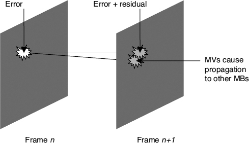
Figure 2.16 Propagation of errors in inter frames

The main profile is intended for digital television broadcasting and next-generation DVD applications, and does not stress error-resilience techniques. However, the extended profile targets streaming video, and includes features to improve error resilience by using data partitioning, and to facilitate switching between different bitstreams by using SP/SI slices. The extended profile also supports all the error-resilience tools of the baseline profile.

2.4.8.1 Slices

H.264 supports picture segmentation in the form of slices. A slice consists of an integer number of MBs of one picture, ranging from a single MB per slice to all MBs of a picture per slice. The segmentation of a picture into slices facilitates the adaptation of the coded slice size to different MTU (maximum transmission unit) sizes and helps to implement schemes such as interleaved packetization [22]. Each slice carries all the information required to decode the MBs it contains.

2.4.8.2 Parameter Sets

The parameter set is a mandatory encoding tool, whose intelligent use greatly enhances error resilience. A parameter set consists of all information related to all the slices of a picture. A number of predefined parameter sets are available at the encoder and the decoder. The encoder chooses a suitable parameter set by referencing the storage location, and the same reference number is included in the slice header of each coded slice to inform the decoder. In this way, in an error-prone environment it is ensured that the most important parameter information arrives with minimum errors [21].

2.4.8.3 Flexible Macroblock Ordering

FMO is a powerful error-resilience tool that allows MBs to be assigned to slices in an order other than the scan order [23, 24]. A Macroblock Allocation map (MBAmap) is used to statically assign each MB to a slice group. All MBs within a slice group are coded using the normal scan order. A maximum of eight slice groups can be used. FMO consists of seven different types, named type 0 to type 6. Each type except type 6 contains a certain pattern, as shown in Figure 2.17. Slice type 0 divides the frame into a number of different sizes of slice group. As the number of slice groups is increased, the number of MBs surrounding each MB increases. For example, slice type 1 spreads the MB into more than one slice group in such a way that each MB is surrounded by MBs from different slice groups. Slice type 2 is used to highlight the regions of interest inside the frame. Slice types 3–5 allow formation of dynamic slice groups in a cyclic order. If a slice group is lost during transmission, reconstruction of the missing blocks is easier with the help of the information in the surrounding MBs. However, FMO reduces the coding efficiency and has high overheads in the form of the MBAmap which has to be transmitted.

Figure 2.17 Different types of FMO in H.264. (a) type 0, (b) type 1, (c) type 2, (d) type 3, (e) type 4, (f) type 5

2.4.8.4 Redundant Slices

RSs have been introduced to support highly-error-prone wireless environments [25]. One or more redundant copies of the MBs, in addition to the coded MBs, are included in a single bitstream. The redundant representation can be coded using different coding parameters. The primary representation is coded at high quality, and the RS representations can be coded at a low quality, utilizing fewer bits. If no error occurs during transmission, the decoder reconstructs only the primary slice and discards all redundant slices. However, if the primary slice is lost during transmission, the decoder uses the information from the redundant slices, if they are available.

2.4.8.5 H.264 Data Partitioning

Data partitioning separates the coded slice data into more than one partition. In contrast to MPEG-4, separate bit strings are created without the need of boundary markers. Each partition has its own header and is transmitted independently according to the assigned priority. H.264 supports three different types of partition:

• Type A partition: the most important information in a video slice, including header data and motion vectors, constitutes the type A partition. Without this information, symbols of other partitions cannot be decoded.
• Type B partition: compromises the INTRA coefficients of a slice. It carries less importance than the type A partition.
• Type C partition: only INTER coefficients and related data are included in the type C partition. This is the least important and the biggest partition.

Data partitioning can be used in Unequal Error Protection (UEP) schemes. For example, the type A partition can be protected more than the other two types. However, if INTER or INTRA partitioning is not available, the decoder can still use the header and motion information to improve the efficiency of error concealment [26, 27].