9.4 User-centric Radio Resource Management in UTRAN
(Portion reprinted, with permission, from O. Abdul Hameed, S. Nasir, H. Karim, T. Masterton, A.M. Kondoz, “Enhancing wireless video transmissions in virtual collaboration environments”, Mobile and Wireless Communications Summit, 2007. 16th IST, vol., no., pp.1–5, 1–5 July 2007. ©2007 IEEE.)
9.4.1 Enhanced Call-admission Control Scheme
In this section, an enhanced power-based downlink call-admission control scheme is presented. The aim of this scheme is to improve the blocking probability for high-priority new call requests such as emergency services call requests. The scheme was designed based on radio resource management works in [57,58]. It takes the user input into account at call-admission control time. The user input is obtained by classifying the new call requests, according to how much they are willing to pay for the services, into three service classes, being Enhanced, Moderate, and Normal. For each new call request, the new call's service class is generated as 50 % for Normal, 30 % for Moderate, and 20 % for Enhanced. The scheme adopts quality optimization using QoS renegotiation or a pre-agreed service level agreement (SLA) such that lower-priority existing calls can give their radio network resources to higher-priority new call requests. Each user has a service quality profile for each traffic type, such as voice, video, or data, that defines maximum and minimum data rates. The scheme is illustrated in Figure 9.54.
A new call request is accepted if there are enough radio network resources available. If not, the new call request's service class is checked. If it is Enhanced, for example, the network tries first to step down the bit rate of Normal-service-class existing calls by the predefined SLA. If enough resources can be obtained after this step, the call is accepted. If not, the same process is applied on existing Moderate-service-class calls. If enough resources are still not available, the new call request is blocked.
9.4.2 Implementation of UTRAN System-level Simulator
A system-level simulator for UMTS terrestrial radio access network (UTRAN) was implemented using the C + + programming language. The simulator's features and functionalities are described below.
9.4.2.1 Cell Layout
The simulated network area models a macro-cellular environment for the uplink and downlink directions [8]. The network topology consists of 49 hexagonal cells that are laid on a wraparound surface to avoid border effects, and hence each cell will have 6 neighbors, as shown in Figure 9.55. The cell radius is 300 m and an omnidirectional antenna is placed at the center of each cell, with one 5 MHz carrier (2100 MHz band) with reuse of one.
9.4.2.2 Traffic Generation
The traffic models adopted in the simulator are for real-time services for voice and video. New call requests arrive at the 49 cell system according to a Poisson process of rate λ call requests/second.

Figure 9.54 Flow chart illustrating the enhanced call-admission control scheme
For homogeneous load, the call requests (or user arrivals) are uniformly distributed over the simulated network area. For hot-spot simulations, about one quarter of the entire system's new call requests will be initiated 10 m below the antenna in the hot-spot cell. No user mobility is considered.
The inter arrival time between two consecutive call requests is exponentially distributed. The call duration is also exponentially distributed with mean call duration of 180 s. To generate the inter arrival times and the call durations the following approach is used:
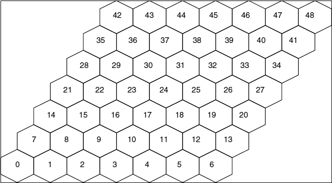
Figure 9.55 Toroidal (wraparound) 49 cell system
Let x be a random variable that follows an exponential distribution with rate α. The random variable x can be generated using the following equation:
where u is a uniformly-distributed random variable between 0 and 1.
To generate the inter arrival times, λ call requests/second is used for the rate parameter α. To generate the call duration times, μ is used for the rate parameter α.
9.4.2.3 Propagation Model
The propagation model adopted in the simulator includes large-scale fading, small-scale fading, and shadow fading. The attenuation between a mobile and the transmit antenna of a cell site, or between a mobile and each of the receiving antennas of a cell site, is modeled by:

where g2 is an exponentially-distributed random variable with unit mean, which accounts for Rayleigh fading; s is a Gaussian random variable with zero mean and a standard deviation of 5 dB, which introduces log normal shadowing due to the terrain irregularities; and L is the path loss.
If the power transmitted from a NodeB towards a mobile is PTX, the power received at the mobile is PRX and is given by:
Fast-fading Model
The fast fading is modeled using an exponentially-distributed random variable with unit mean, which accounts for Rayleigh fading [57].
Path-loss Model
The path-loss component of the propagation model is calculated according to the path loss model for the vehicular test environment [8] as:
where R is the NodeB–mobile separation in kilometers.
Shadow-fading Model
The shadow-fading component of the propagation model is modeled as a Gaussian-distributed random variable with zero mean and standard deviation σ.Xi may be expressed as the weighted sum of a component Z common to all cell sites and a component Zi that is independent from one cell site to the next. Both components are assumed to be Gaussian-distributed random variables with zero mean and standard deviation σ independent from each other, so that:
such that a2 + b2 = 1.
Typical parameters are σ = 8.9 and a2 = b2 = 1/2 for 50% correlation. The correlation is 0.5 between sectors from different cells, and 1.0 between sectors of the same cell [59].
9.4.2.4 Interference
The interference consists of three parts, being intra-cell interference, inter-cell interference, and thermal noise power. Intra-cell interference IOWN is the interference generated by users that are connected to the same base station. IOWN also includes interference caused by the perch channel and common channels, and their transmission powers are in total equal to 30 dBm for macro-cells [60]. Inter-cell interference IOTHER is the interference generated from the other cells. Thermal noise power N0 is equal to −99 dBm and is calculated for the 4.096 MHz band by assuming a 9 dB system noise figure.
9.4.2.5 Signal-to-interference Ratio (SIR)
The signal-to-interference ratio (SIR) in the downlink direction at the user after dispreading is calculated every 10 ms for each active user in the simulator as:

where S is the received signal, GP is the processing gain (or SF), IOWN is the intra-cell interference, IOTHER is the inter-cell interference, and α is the orthogonality factor, which takes into account the fact that the downlink is not perfectly orthogonal due to multipath propagation. An orthogonality factor of 0 corresponds to perfectly orthogonal intra-cell users, while with a value of 1 the intra-cell interference has the same effect as inter-cell interference.
9.4.2.6 Power Control
The downlink traffic channels are power-controlled using a simple SIR-based fast-inner-loop power control in order to maintain the SIR at a target value. Perfect power control is assumed, i. e. during the power-control loop each downlink traffic channel perfectly achieves the Eb/No target, assuming that the maximum NodeB transmission power is not exceeded. With the assumption of perfect power control, power-control error is assumed equal to 0% and power-control delay is assumed to be 0 seconds. UEs whose downlink traffic channel is not able to achieve the Eb/N0 target at the end of a power-control loop are considered in outage.
Initial transmission power for the power-control loop of the downlink traffic channel is chosen randomly in the transmission power range. However, the initial transmission power should not affect the convergence process (power-control loop) to the target Eb/N0. Here it is assumed that the power control operates at a frequency of 100 Hz for faster simulations. The new power level is evaluated as:
where PTX(t−1) is the transmitting power of the link in the (t − 1)th step of the simulation. The maximum power for each downlink traffic channel is 30 dBm in a macro-cellular environment [60], and if the power control requires a power higher than the maximum value, the maximum value is adopted. In addition, if the sum of the powers required by the downlink channels exceeds the NodeB maximum transmission power, all the powers are proportionally reduced to limit the total power at the maximum value.
9.4.2.7 Call-admission Control (CAC)
The call-admission control (CAC) scheme used in the simulator was a power-based CAC scheme that estimates the load of the radio network during the admission of a new call request generated by a user. The total power transmitted from the NodeB is a parameter that can be used to estimate the network load in downlink direction. A new call request is accepted as long as the output power level at the consulted NodeB stays below a certain predefined threshold.
If the total power transmitted from a NodeB is Ptotal and the maximum downlink transmission power of the NodeB is Pmax, a new call request to this NodeB will be accepted if:

and will be blocked if:

The idea of considering the ratio Ptotal/Pmax instead of the absolute threshold value Pthr is based on the assumption that it would be easier in a real system to have a simple tuning criterion based on a relative threshold [57]. The value of the threshold varies in the interval [0,1].
9.4.2.8 Performance Metrics
The system's performance is evaluated using a number of performance metrics. The following parameters are obtained from the system-level simulator's output:
- Number of new call requests.
- Number of accepted call requests.
- Number of blocked call requests.
- Number of quality dropped calls.
- New-call-blocking probability (Pblocking), which is defined as the number of blocked call requests divided by the number of generated call requests. Blocking occurs if a new call request is denied access to the system.
- Call-dropping probability (Pdropping), which is defined as the number of dropped calls divided by the number of accepted calls. After each power-control loop the actual SIR values experienced by each connection are evaluated, and dropping occurs when a connection's SIR is more than 3 dB below the value of SIRtarget.
- Accepted traffic (erlangs/cell), which is defined as the mean number of active calls per cell.
9.4.2.9 Simulation Techniques
The steady-state simulation technique was used for the system-level simulations using the implemented system-level simulator. To gather steady-state simulation output requires statistical assurance that the simulation model has reached the steady-state. The main difficulty is to obtain independent simulation runs with the exclusion of the transient period. The two techniques commonly used for steady-state simulation are the method of batch means and the method of independent replication. Neither of these methods is superior in all cases. Their performance depends on the magnitude of the traffic intensity [61].
Method of Batch Means
This method involves only one very long simulation run, which is subdivided into an initial transient period and n batches, as shown in Figure 9.56. Each batch is then treated as an independent run of the simulation experiment. No observations are made during the transient period, which is treated as a warm-up interval. Choosing a large batch interval size would effectively lead to independent batches and hence independent runs of the simulation; however, since the number of batches is small, one cannot invoke the central limit theorem to construct the needed confidence interval. On the other hand, choosing a small batch interval size would effectively lead to significant correlation between successive batches, therefore the results cannot be applied in constructing an accurate confidence interval.
Suppose you have n equal batches of m observations each. The means of each batch is:
The overall estimate is:


Figure 9.56 Method of batch means
The 100(1 − α/2)% confidence interval using the Z-table (or T-table for n less than, say, 30) is:
where the variance is:

Method of Independent Replications
This method is the most popularly used for systems with a short transient period. This method requires independent runs of the simulation experiment for different initial random seeds of the simulator's random number generator. For each independent replication of the simulation run its transient period is removed, as shown in Figure 9.57. For the observed intervals after the transient period, data is collected and processed for the point estimates of the performance measure and for its subsequent confidence interval.

Figure 9.57 Method of independent replications
Suppose you have n replications with m observations each. The means of each replication is:

The overall estimate is:
The 100(1 − α/2)% confidence interval using the Z-table (or T-table for n less than, say, 30) is:
where the variance is:

In the simulations, we have adopted the method of independent replications.
9.4.3 Performance Evaluation of Enhanced CAC Scheme
In order to evaluate the performance of the enhanced power-based CAC in the downlink direction, steady-state static system-level simulations were conducted using the implemented system-level simulator. Two kinds of stream services were considered in the simulations, being voice and video. The following traffic scenarios were considered:
- Voice only: AMR voice service at 12.2 and 5.15 kbps using SFs of 128 and 256, respectively.
- Video only: H.264/AVC video at 64 and 128 kbps using SFs of 32 and 16, respectively.
The simulation time was set to 100 000 timeslots (each timeslot is of 10 ms duration) for each offered traffic value, and each simulation run was repeated 10 times and the average was taken. The results were collected after a warm-up period that was found to be 60 000 timeslots (or equivalently 600 s). The simulation parameters used in the system-level experiments are listed in Table 9.28.
Table 9.28 System-level simulation parameters
| Radio Access | WCDMA FDD downlink |
| Environment | Vehicular A |
| Chip Rate | 3.84 Mcps |
| Carrier Frequency | 2.0 GHz |
| Bandwidth | 5.0 MHz |
| Orthogonality Factor | 0.4 |
| Maximum NodeB Transmission Power | 43 dBm |
| Perch Channel and Common Channels Power | 30 dBm |
| Thermal Noise Power (Downlink) | −99 dBm |
| Cell Radius | 300m |
| Log Normal Shadowing | Mean = 0 dB, standard deviation = 5 dB |

Figure 9.58 Accepted traffic versus offered traffic for different traffic types and data rates
The first set of experiments was conducted to validate the system-level simulator. The traffic scenario considered was a voice service at 12.2 kbps using an SF of 128 for a CAC threshold value of 0.5. The simulation results are presented in Figure 9.58, which shows the accepted traffic versus the offered traffic curves in erlangs/cell for a 49 cell system and two different traffic types, being voice and video.
The simulator's performance was validated with [56]. The top two curves represent the accepted traffic in erlangs/cell versus the offered traffic in erlangs/cell for an all-voice traffic scenario at 12.2kbps. The “original_0.5” in the figure's legend represents the performance obtained in [56], whereas the “voice, SF = 128, CAC_thr = 0.5 (validation)” represents the performance obtained using the implemented simulator.
The bottom three curves are for video-only traffic at different data rates. The top one is for video traffic at 64 kbps, the bottom one for video at 128 kbps, whereas the middle one is obtained when using the scheme. The figure shows that, using the scheme, the accepted traffic is improved (or equivalently, lower blocking probability has been achieved) for video traffic users that have been classified into the three service classes. Therefore, the scheme can be used to provide lower blocking probability for the high-priority users, achieving the expected end-to-end QoS.