
Chapter 27
Genetic Algorithms
27.1 Introduction To Genetic Algorithms
Genetic algorithms (GAs) attempt to computationally mimic the processes by which natural selection operates, and apply them to solve business and research problems. Developed by John Holland in the 1960s and 1970s (Holland1), GAs provide a framework for studying the effects of such biologically inspired factors as mate selection, reproduction, mutation, and crossover of genetic information.
In the natural world, the constraints and stresses of a particular environment force the different species (and different individuals within species) to compete to produce the fittest offspring. In the world of GAs, the fitness of various potential solutions is compared, and the fittest potential solutions evolve to produce ever more optimal solutions.
Not surprisingly, the field of GAs has borrowed heavily from genomic terminology. Each cell in our body contains the same set of chromosomes, strings of DNA that function as a blueprint for making one of us. Then, each chromosome can be partitioned into genes, which are blocks of DNA designed to encode a particular trait such as eye color. A particular instance of the gene (e.g., brown eyes) is an allele. Each gene is to be found at a particular locus on the chromosome. Recombination, or crossover, occurs during reproduction, where a new chromosome is formed by combining the characteristics of both parents' chromosomes. Mutation, the altering of a single gene in a chromosome of the offspring, may occur, randomly and relatively rarely. The offspring's fitness is then evaluated, either in terms of viability (living long enough to reproduce) or in the offspring's fertility.
Now, in the field of GAs, a chromosome refers to one of the candidate solutions to the problem, a gene is a single bit or digit of the candidate solution, and an allele is a particular instance of the bit or digit (e.g., 0 for binary-encoded solutions or the number 7 for real-valued solutions). Recall that binary numbers have base two, so that the first “decimal” place represents “ones,” the second represents “twos,” the third represents “fours,” the fourth represents “eights,” and so forth. So the binary string 10101010 represents
in decimal notation.
There are three operators used by GAs, selection, crossover, and mutation.
- Selection. The selection operator refers to the method used for selecting which chromosomes will be reproducing. The fitness function evaluates each of the chromosomes (candidate solutions), and the fitter the chromosome, the more likely it will be selected to reproduce.
- Crossover. The crossover operator performs recombination, creating two new offspring by randomly selecting a locus and exchanging subsequences to the left and right of that locus between two chromosomes chosen during selection. For example, in binary representation, two strings 11111111 and 00000000 could be crossed over at the sixth locus in each to generate the two new offspring 11111000 and 00000111.
- Mutation. The mutation operator randomly changes the bits or digits at a particular locus in a chromosome, usually, however with very small probability. For example, after crossover, the 11111000 child string could be mutated at locus two to become 10111000. Mutation introduces new information to the genetic pool, and protects against converging too quickly to a local optimum.
Most GAs function by iteratively updating a collection of potential solutions, called a population. Each member of the population is evaluated for fitness on each cycle. A new population then replaces the old population using the above operators, with the fittest members being chosen for reproduction or cloning. The fitness function ![]() is a real-valued function operating on the chromosome (potential solution), not the gene, so that the x in
is a real-valued function operating on the chromosome (potential solution), not the gene, so that the x in ![]() refers to the numeric value taken by the chromosome at the time of fitness evaluation.
refers to the numeric value taken by the chromosome at the time of fitness evaluation.
27.2 Basic Framework of a Genetic Algorithm
The following introductory GA framework is adapted from Mitchell2 in her interesting book An Introduction to Genetic Algorithms.
- Step 0. Initialization. Assume that the data are encoded in bit strings (1's and 0's). Specify a crossover probability or crossover rate
 , and a mutation probability or mutation rate
  . Usually,
  is chosen to be fairly high (e.g., 0.7), and
  is chosen to be very low (e.g., 0.001).
 - Step 1. The population is chosen, consisting of a set of n chromosomes, each of length l.
- Step 2. The fitness
 for each chromosome in the population is calculated.
 - Step 3. Iterate through the following steps until n offspring have been generated.
- Step 3a. Selection. Using the values from the fitness function
 from step 2, assign a probability of selection to each individual chromosome, with higher fitness providing a higher probability of selection. The usual term for the way these probabilities are assigned is the roulette wheel method. For each chromosome
  , find the proportion of this chromosome's fitness to the total fitness summed over all the chromosomes. That is, find
  , and assign this proportion to be the probability of selecting that chromosome for parenthood. Each chromosome then has a proportional slice of the putative roulette wheel spun to choose the parents. Then select a pair of chromosomes to be parents, based on these probabilities. Allow the same chromosome to be potentially selected to be a parent more than once. Allowing a chromosome to pair with itself will generate three copies of that chromosome to the new generation. If the analyst is concerned about converging too quickly to a local optimum, then perhaps such pairing should not be allowed.
 - Step 3b. Crossover. Select a randomly chosen locus (crossover point) for where to perform the crossover. Then, with probability
 , perform crossover with the parents selected in step 3a, thereby forming two new offspring. If the crossover is not performed, clone two exact copies of the parents to be passed on to the new generation.
 - Step 3c. Mutation. With probability
 , perform mutation on each of the two offspring at each locus point. The chromosomes then take their place in the new population. If n is odd, discard one new chromosome at random.
- Step 3a. Selection. Using the values from the fitness function
- Step 4. The new population of chromosomes replaces the current population.
- Step 5. Check whether termination criteria have been met. For example, is the change in mean fitness from generation to generation vanishingly small? If convergence is achieved, then stop and report results; otherwise, go to step 2.
Each cycle through this algorithm is called a generation, with most GA applications taking from 50 to 500 generations to reach convergence. Mitchell suggests that researchers try several different runs with different random number seeds, and report the model evaluation statistics (e.g., best overall fitness) averaged over several different runs.
27.3 Simple Example of a Genetic Algorithm at Work
Let us examine a simple example of a GA at work. Suppose our task is to find the maximum value of the normal distribution with mean ![]() and standard deviation
and standard deviation ![]() (Figure 27.1). That is, we would like to find the maximum value of:
(Figure 27.1). That is, we would like to find the maximum value of:

Figure 27.1 Find the maximum value of the normal(16, 4) distribution.
We allow X to take on only the values described by the first five binary digits; that is, 00000 through 11111, or 0–31 in decimal notation.
27.3.1 First Iteration
- Step 0. Initialization. We define the crossover rate to be
 and the mutation rate to be
  .
. - Step 1. Our population will be a set of four chromosomes, randomly chosen from the set 00000–11111. So, n = 4 and l = 5. These are 00100 (4), 01001 (9), 11011 (27), and 11111 (31).
- Step 2. The fitness
 for each chromosome in the population is calculated.
 - Step 3. Iterate through the following steps until n offspring have been generated.
-
Step 3a. Selection. We have the sum of the fitness values equal to

Then, the probability that each of our chromosomes will be selected for parenthood is found by dividing their value for
 by the sum 0.025038. These are also shown in Table 27.1. Clearly, chromosome 01001 gets a very large slice of the roulette wheel! The random selection process gets underway. Suppose that chromosomes 01001 and 11011 are selected to be the first pair of parents, because these are the two chromosomes with the highest fitness.
Table 27.1 Fitness and probability of selection for each chromosome
Chromosome Decimal Value Fitness Selection Probability 00100 4 0.001108 0.04425 01001 9 0.021569 0.86145 11011 27 0.002273 0.09078 11111 31 0.000088 0.00351 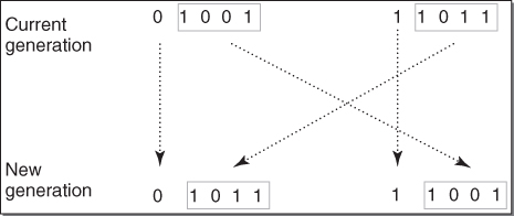
Figure 27.2 Performing crossover at locus two on the first two parents.
- Step 3b. Crossover. The locus is randomly chosen to be the second position. Suppose the large crossover rate of
 , 0.75, leads to crossover between 01001 and 11011 occurring at the second position. This is shown in Figure 27.2. Note that the strings are partitioned between the first and the second bits. Each child chromosome receives one segment from each of the parents. The two chromosomes thus formed for the new generation are 01011 (11) and 11001 (25).
 - Step 3c. Mutation. Because of the low mutation rate, suppose that none of the genes for 01011 or 11001 are mutated. We now have two chromosomes in our new population. We need two more, so we cycle back to step 3a.
- Step 3a. Selection. Suppose that this time chromosomes 01001 (9) and 00100 (4) are selected by the roulette wheel method.
- Step 3b. Crossover. However, this time suppose that crossover does not take place. Thus, clones of these chromosomes become members of the new generation, 01001 and 00100. We now have n = 4 members in our new population.
-
- Step 4. The new population of chromosomes therefore replaces the current population.
- Step 5. And we iterate back to Step 2.
27.3.2 Second Iteration
- Step 2. The fitness
 for each chromosome in the population is calculated, as shown in Table 27.2.
- Step 3a. Selection. The sum of the fitness values for the second generation is
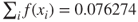 , which means that the average fitness among the chromosomes in the second generation is three times that of the first generation. The selection probabilities are calculated, and shown in Table 27.2.
- Step 3a. Selection. The sum of the fitness values for the second generation is
Table 27.2 Fitness and probability of selection for the second generation
| Chromosome | Decimal Value | Fitness | Selection Probability |
| 00100 | 4 | 0.001108 | 0.014527 |
| 01001 | 9 | 0.021569 | 0.282783 |
| 01011 | 11 | 0.045662 | 0.598657 |
| 11001 | 25 | 0.007935 | 0.104033 |
We ask you to continue this example in the exercises.
27.4 Modifications and Enhancements: Selection
For the selection operator, the analyst should be careful to balance fitness with diversity. If fitness is favored over variability, then a set of highly fit but suboptimal chromosomes will dominate the population, reducing the ability of the GA to find the global optimum. If diversity is favored over fitness, then model convergence will be too slow.
For example, in the first generation above, one particular gene 01001 (9) dominated the fitness measure, with over 86% of the selection probability. This is an example of selection pressure, and a potential example of the crowding phenomenon in GAs, where one particular chromosome that is much fitter than the others begins to reproduce, generating too many clones and similar copies of itself in future generations. By reducing the diversity of the population, crowding impairs the ability of the GA to continue to explore new regions of the search space.
A variety of techniques are available to handle crowding. De Jong3 suggested that new generation chromosomes should replace the individual most similar to itself in the current generation. Goldberg and Richardson4 posited a fitness sharing function, where a particular chromosome's fitness was decreased by the presence of other similar population members, where the more similarity, the greater the decrease. Thus, diversity was rewarded.
Changing the mating conditions can also be used to increase population diversity. Deb and Goldberg5 showed that if mating can take place only between sufficiently similar chromosomes, then distinct “mating groups” will have a propensity to form. These groups displayed low within-group variation and high between-group variation. However, Eshelman6 and Eshelman and Schaffer7 investigated the opposite strategy by not allowing matings between chromosomes that were sufficiently alike. The result was to maintain high variability within the population as a whole.
Sigma scaling, proposed by Forrest,8 maintains the selection pressure at a relatively constant rate, by scaling a chromosome's fitness by the standard deviation of the fitnesses. If a single chromosome dominates at the beginning of the run, then the variability in fitnesses will also be large, and scaling by the variability will reduce the dominance. Later in the run, when populations are typically more homogeneous, scaling by this smaller variability will allow the highly fit chromosomes to reproduce. The sigma-scaled fitness is as follows:
where ![]() and
and ![]() refer to the mean fitness and standard deviation of the fitnesses for the current generation.
refer to the mean fitness and standard deviation of the fitnesses for the current generation.
Boltzmann selection varies the selection pressure, depending on how far along in the run the generation is. Early on, it may be better to allow lower selection pressure, allowing the less-fit chromosomes to reproduce at rates similar to the fitter chromosomes, and thereby maintaining a wider exploration of the search space. Later on in the run, increasing the selection pressure will help the GA to converge more quickly to the optimal solution, hopefully the global optimum. In Boltzmann selection, a temperature parameter T is gradually reduced from high levels to low levels. A chromosome's adjusted fitness is then found as follows:
As the temperature falls, the difference in expected fitness increases between high-fit and low-fit chromosomes.
Elitism, developed by De Jong, refers to the selection condition requiring that the GA retain a certain number of the fittest chromosomes from one generation to the next, protecting them against destruction through crossover, mutation, or inability to reproduce. Michell, Haupt, and Haupt9 and others report that elitism greatly improves GA performance.
Rank selection ranks the chromosomes according to fitness. Ranking avoids the selection pressure exerted by the proportional fitness method, but it also ignores the absolute differences among the chromosome fitnesses. Ranking does not take variability into account, and provides a moderate adjusted fitness measure, because the difference in probability of selection between chromosomes ranked k and k + 1 is the same, regardless of the absolute differences in fitness.
Tournament ranking is computationally more efficient than rank selection, while preserving the moderate selection pressure of rank selection. In tournament ranking, two chromosomes are chosen at random and with replacement from the population. Let c be a constant chosen by the user to be between zero and one (e.g., 0.67). A random number r, ![]() , is drawn. If r < c, then the fitter chromosome is selected for parenthood; otherwise, the less-fit chromosome is selected.
, is drawn. If r < c, then the fitter chromosome is selected for parenthood; otherwise, the less-fit chromosome is selected.
27.5 Modifications and Enhancements: Crossover
27.5.1 Multi-Point Crossover
The single-point crossover operator that we have outlined here suffers from what is known as positional bias. That is, the performance of the GA depends, in part, on the order that the variables occur in the chromosome. So, genes in loci 1 and 2 will often be crossed over together, simply because of their proximity to each other, whereas genes in loci 1 and 7 will rarely cross over together. Now, if this positioning reflects natural relationships within the data and among the variables, then this is not such a concern, but such a priori knowledge is relatively rare.
The solution is to perform multi-point crossover, as follows. First, randomly select a set of crossover points, and split the parent chromosomes at those points. Then, to form the children, recombine the segments by alternating between the parents, as illustrated in Figure 27.3.
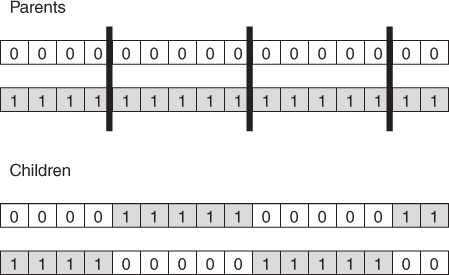
Figure 27.3 Multi-point crossover.
27.5.2 Uniform Crossover
Another alternative crossover operator is uniform crossover. In uniform crossover, the first child is generated as follows. Each gene is randomly assigned to be that of either one or the other parent, with 50% probability. The second child would then take the inverse of the first child. One advantage of uniform crossover is that the inherited genes are independent of position. Uniform crossover is illustrated in Figure 27.4. A modified version of uniform crossover would be to allow the probabilities to depend on the fitness of the respective parents.
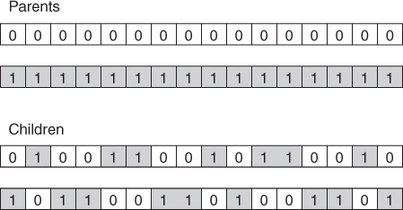
Figure 27.4 Uniform crossover.
Eiben and Smith10 discuss the roles of crossover and mutation, and the cooperation and competition between them with respect to the search space. They describe crossover as explorative, discovering promising new regions in the search space by making a large jump to a region between the two parent areas. And they describe mutation as exploitative, optimizing present information within an already discovered promising region, creating small random deviations and thereby not wandering far from the parents. Crossover and mutation complement each other, because only crossover can bring together information from both parents, and only mutation can introduce completely new information.
27.6 Genetic Algorithms for Real-Valued Variables
The original framework for GAs was developed for binary-encoded data, because the operations of crossover and mutation worked naturally and well with such data. However, most data mining data come in the form of real numbers, often with many decimals worth of precision.
Some analysts have tried quantizing the real-valued (continuous) data into binary form. However, to re-express the real-valued data in binary terms will necessarily result in a loss of information, due to the degradation in precision caused by rounding to the nearest binary digit. To combat this loss in precision, each binary chromosome would need to be made longer, adding digits that will inevitably impair the speed of the algorithm.
Therefore, methods for applying GAs directly to real-valued data have been investigated. Eiben and Smith suggest the following methods for performing the crossover operation.
27.6.1 Single Arithmetic Crossover
Let the parents be ![]() and
and ![]() . Pick the kth gene at random. Then, let the first child be of the form
. Pick the kth gene at random. Then, let the first child be of the form ![]() , and the second child be of the form
, and the second child be of the form ![]() , for
, for ![]() .
.
For example, let the parents be ![]() and
and ![]() , let
, let ![]() , and select the third gene at random. Then, single arithmetic crossover would produce the first child to be
, and select the third gene at random. Then, single arithmetic crossover would produce the first child to be
and the second child to be
27.6.2 Simple Arithmetic Crossover
Let the parents be ![]() and
and ![]() . Pick the kth gene at random, and mix values for all genes at this point and beyond. That is, let the first child be of the form
. Pick the kth gene at random, and mix values for all genes at this point and beyond. That is, let the first child be of the form ![]() , and the second child be of the form
, and the second child be of the form ![]() , for
, for ![]() .
.
For example, let the parents be ![]() and
and ![]() , let
, let ![]() , and select the third gene at random. Then, simple arithmetic crossover would produce the first child to be
, and select the third gene at random. Then, simple arithmetic crossover would produce the first child to be
and the second child to be
27.6.3 Whole Arithmetic Crossover
Let the parents be ![]() and
and ![]() . Perform the above mixture to the entire vector for each parent. The calculation of the child vectors is left as an exercise. Note that, for each of these arithmetic crossover techniques, the affected genes represent intermediate points between the parents' values, with
. Perform the above mixture to the entire vector for each parent. The calculation of the child vectors is left as an exercise. Note that, for each of these arithmetic crossover techniques, the affected genes represent intermediate points between the parents' values, with ![]() generating the mean of the parents' values.
generating the mean of the parents' values.
27.6.4 Discrete Crossover
Here, each gene in the child chromosome is chosen with uniform probability to be the gene of one or the other of the parents' chromosomes. For example, let the parents be ![]() and
and ![]() , one possible child could be
, one possible child could be ![]() , with the third gene coming directly from the first parent and the others coming from the second parent.
, with the third gene coming directly from the first parent and the others coming from the second parent.
27.6.5 Normally Distributed Mutation
To avoid converging too quickly toward a local optimum, a normally distributed “random shock” may be added to each variable. The distribution should be normal, with a mean of zero, and a standard deviation of ![]() , which controls the amount of change (as most random shocks will lie within one
, which controls the amount of change (as most random shocks will lie within one ![]() of the original variable value). If the resulting mutated variable lies outside the allowable range, then its value should be reset so that it lies within the range. If all variables are mutated, then clearly
of the original variable value). If the resulting mutated variable lies outside the allowable range, then its value should be reset so that it lies within the range. If all variables are mutated, then clearly ![]() in this case.
in this case.
For example, suppose the mutation distribution is ![]() , and that we wish to apply the mutation to the child chromosome from the discrete crossover example,
, and that we wish to apply the mutation to the child chromosome from the discrete crossover example, ![]() . Assume that the four random shocks generated from this distribution are 0.05, −0.17, −0.03, and 0.08. Then, the child chromosome becomes
. Assume that the four random shocks generated from this distribution are 0.05, −0.17, −0.03, and 0.08. Then, the child chromosome becomes ![]() .
.
27.7 Using Genetic Algorithms to Train a Neural Network
A neural network consists of a layered, feed-forward, completely connected network of artificial neurons, or nodes. Neural networks are used for classification or estimation. See Mitchell,11 Fausett,12 Haykin,13 Reed and Marks,14 or Chapter 12 of this book for details on neural network topology and operation. Figure 27.5 provides a basic diagram of a simple neural network.

Figure 27.5 A simple neural network.
The feed-forward nature of the network restricts the network to a single direction of flow, and does not allow looping or cycling. The neural network is composed of two or more layers, although most networks consist of three layers, an input layer, a hidden layer, and an output layer. There may be more than one hidden layer, although most networks contain only one, which is sufficient for most purposes. The neural network is completely connected, meaning that every node in a given layer is connected to every node in the next layer, although not to other nodes in the same layer. Each connection between nodes has a weight (e.g., W1A) associated with it. At initialization, these weights are randomly assigned to values between zero and one.
How does the neural network learn? Neural networks represent a supervised learning method, requiring a large training set of complete records, including the target variable. As each observation from the training set is processed through the network, an output value is produced from the output node (assuming we have only one output node). This output value is then compared to the actual value of the target variable for this training set observation, and the error ![]() is calculated. This prediction error is analogous to the residuals in regression models. To measure how well the output predictions are fitting the actual target values, most neural network models use the sum of squared errors:
is calculated. This prediction error is analogous to the residuals in regression models. To measure how well the output predictions are fitting the actual target values, most neural network models use the sum of squared errors:
where the squared prediction errors are summed over all the output nodes and over all the records in the training set.
The problem is therefore to construct a set of model weights that will minimize this SSE. In this way, the weights are analogous to the parameters of a regression model. The “true” values for the weights that will minimize SSE are unknown, and our task is to estimate them, given the data. However, due to the nonlinear nature of the sigmoid functions permeating the network, there exists no closed-form solution for minimizing SSE, as there exists for least-squares regression. Most neural network models therefore use backpropagation, a gradient-descent optimization method, to help find the set of weights that will minimize SSE. Backpropagation takes the prediction error ![]() for a particular record, and percolates the error back through the network, assigning partitioned “responsibility” for the error to the various connections. The weights on these connections are then adjusted to decrease the error, using gradient descent.
for a particular record, and percolates the error back through the network, assigning partitioned “responsibility” for the error to the various connections. The weights on these connections are then adjusted to decrease the error, using gradient descent.
However, as finding the best set of weights in a neural network is an optimization task, GAs are wonderfully suited to do so. The drawbacks of backpropagation include the tendency to become stuck at local minima (as it follows a single route through the weight space) and the requirement to calculate derivative or gradient information for each weight. Also, Unnikrishnan et al.15 state that improper selection of initial weights in backpropagation will delay convergence. GAs, however, perform a global search, lessening the chances of becoming caught in a local minimum, although, of course, there can be no guarantees that the global minimum has been obtained. Also, GAs require no derivative or gradient information to be calculated. However, neural networks using GAs for training the weights will run slower than traditional neural networks using backpropagation.
GAs apply a much different search strategy than backpropagation. The gradient-descent methodology in backpropagation moves from one solution vector to another vector that is quite similar. The GA search methodology, however, can shift much more radically, generating a child chromosome that may be completely different than either parent. This behavior decreases the probability that GAs will become stuck in local optima.
Huang, Dorsey, and Boose16 apply a neural network optimized with a GA to forecast financial distress in life insurance companies. Unnikrishnan, Mahajan, and Chu used GAs to optimize the weights in a neural network, which was used to model a three-dimensional ultrasonic positioning system. They represented the network weights in the form of chromosomes, similarly to Table 27.3 for the neural network weights in Figure 27.5. However, their chromosome was 51 weights long, reflecting their 5-4-4-3 topology of five input nodes, four nodes in each of two hidden layers, and three output nodes. The authors cite the length of the chromosome as the reason the model was outperformed both by a backpropagation neural network and a traditional linear model.
Table 27.3 Chromosome representing weights from neural network in Figure 27.5
| W1A | W1B | W2A | W2B | W3A | W3B | W0A | W0B | WAZ | WBZ | W0Z |
David Montana and Lawrence Davis17 provide an example of using GAs to optimize the weights in a neural network (adapted here from Mitchell). Their research task was to classify “lofargrams” (underwater sonic spectrograms) as either interesting or not interesting. Their neural network had a 4-7-10-1 topology, giving a total of 126 weights in their chromosomes. The fitness function used was the usual neural network metric, ![]() , except that the weights being adjusted represented the genes in the chromosome.
, except that the weights being adjusted represented the genes in the chromosome.
For the crossover operator, they used a modified discrete crossover. Here, for each non-input node in the child chromosome, a parent chromosome is selected at random, and the incoming links from the parent are copied to the child for that particular node. Thus, for each pair of parents, only one child is created. For the mutation operator, they used a random shock similar to the normal distribution mutation shown above. Because neural network weights are constrained to lie between −1 and 1, the resulting weights after application of the mutation must be checked that they do not stray outside this range.
The modified discrete crossover is illustrated in Table 27.4 and Figure 27.6. In this example, the weights incoming to Node A are supplied by Parent 1, and the weights incoming to nodes B and Z are supplied by parent 2 (shaded).
Table 27.4 Table of neural network weights indicating results of crossover
| W1A | W1B | W2A | W2B | W3A | W3B | W0A | W0B | WAZ | WBZ | W0Z | |
| Parent 1 | 0.1 | −0.2 | 0.7 | −0.6 | 0.4 | 0.9 | −0.1 | 0.3 | −0.5 | 0.8 | −0.2 |
| Parent 2 | 0.2 | −0.4 | 0.5 | −0.5 | 0.3 | 0.7 | −0.2 | 0.1 | −0.6 | 0.9 | −0.3 |
| Child | 0.1 | −0.4 | 0.7 | −0.5 | 0.4 | 0.7 | −0.1 | 0.1 | −0.6 | 0.9 | −0.3 |
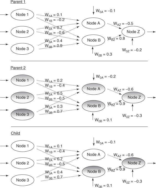
Figure 27.6 Illustrating crossover in neural network weights.
The random shock mutation is illustrated in Table 27.5 and Figure 27.7. In this example, the mutation was applied to the weights incoming to node B only, for the child generated from the crossover operation. The new weights are not far from the old weights. Montana and Davis' GA-based neural network outperformed a backpropagation neural network, despite a total of 126 weights in their chromosomes.
Table 27.5 Weights before and after mutation
| W1A | W1B | W2A | W2B | W3A | W3B | W0A | W0B | WAZ | WBZ | W0Z | |
| Before | 0.1 | −0.4 | 0.7 | −0.5 | 0.4 | 0.7 | −0.1 | 0.1 | −0.6 | 0.9 | −0.3 |
| Shock | None | −0.05 | None | −0.07 | None | 0.02 | None | None | None | None | none |
| After | 0.1 | −0.45 | 0.7 | −0.57 | 0.4 | 0.72 | −0.1 | 0.1 | −0.6 | 0.9 | −0.3 |
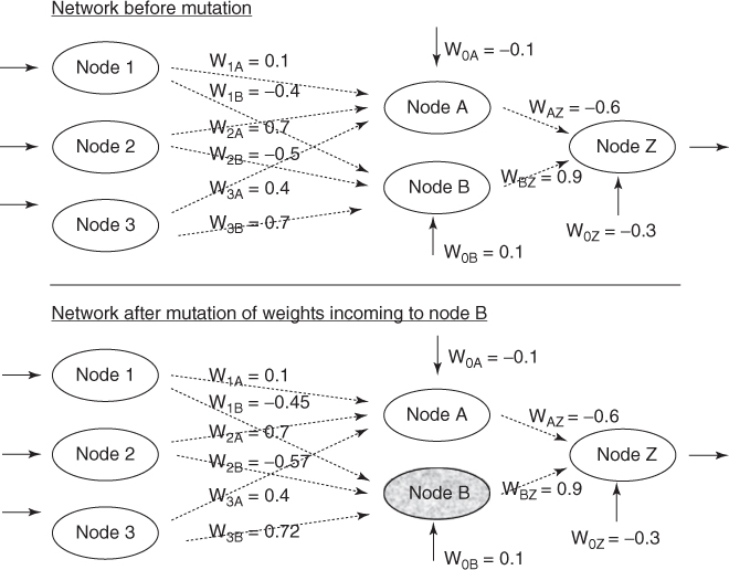
Figure 27.7 Illustrating mutation in neural network weights.
27.8 WEKA: Hands-On Analysis Using Genetic Algorithms
This exercise explores the use of WEKA's Genetic Search class to optimize (choose) a subset of inputs used to classify patients as having either benign or malignant forms of breast cancer. The input file breast_cancer.arff used in our experiment is adapted from the Wisconsin Breast Cancer Database. Breast_cancer.arff contains 683 instances after deleting 16 records containing one or more missing values. In addition, it contains nine numeric inputs (“sample code number” attribute deleted) and a target attribute class that takes on values 2 (benign) and 4 (malignant). Table 27.6 shows the ARFF header and first 10 instances from breast_cancer.arff:
Table 27.6 Breast Cancer Input File breast_cancer.arff
@relation breast_cancer.arff@attribute clump_thickness@attribute uniform_cell_size@attribute uniform_cell_shape@attribute marg_adhesion@attribute single_cell_size@attribute bare_nuclei@attribute bland_chromatin@attribute normal_nucleoli@attribute mitoses@attribute class@data 5,1,1,1,2,1,3,1,1,2 5,4,4,5,7,10,3,2,1,2 3,1,1,1,2,2,3,1,1,2 6,8,8,1,3,4,3,7,1,2 4,1,1,3,2,1,3,1,1,2 8,10,10,8,7,10,9,7,1,4 1,1,1,1,2,10,3,1,1,2 2,1,2,1,2,1,3,1,1,2 2,1,1,1,2,1,1,1,5,2 4,2,1,1,2,1,2,1,1,2... |
numericnumericnumericnumericnumericnumericnumericnumericnumericnumeric{2,4} |
Next, we load the input file and become familiar with the class distribution.
- Click Explorer from the WEKA GUI Chooser dialog.
- On the Preprocess tab, press Open file and specify the path to the input file, breast_cancer.arff.
- Under Attributes (lower left), select the class attribute from the list.
The WEKA Preprocess tab displays the distribution for class, and indicates that 65% (444/683) of the records have value 2 (benign), while the remaining 35% (239/683) have value 4 (malignant), as shown in Figure 27.8.

Figure 27.8 WEKA Explorer: class distribution.
Next, let us establish a baseline and classify the records using naïve Bayes with 10-fold cross-validation, where all nine attributes are input to the classifier.
- Select the Classify tab.
- Under Classifier, press the Choose button.
- Select Classifiers → Bayes → Naïve Bayes from the navigation hierarchy.
- By default, under Test options, notice that WEKA specifies Cross-validation. We will use this option for our experiment because we have a single data file.
- Click Start.
The results in the Classifier output window show that naïve Bayes achieves a very impressive 96.34% (658/683) classification accuracy. This obviously leaves little room for improvement. Do you suppose all nine attributes are equally important to the task of classification? Is there possibly a subset of the nine attributes, when selected as input to naïve Bayes, which leads to improved (or comparable level of) classification accuracy?
Before determining the answers to these questions, let us review WEKA's approach to attribute selection. It is not unusual for real-world data sets to contain irrelevant, redundant, or noisy attributes, which ultimately contribute to degradation in classification accuracy. In contrast, removing nonrelevant attributes often leads to improved classification accuracy. WEKA's supervised attribute selection filter enables a combination of evaluation and search methods to be specified, where the objective is to determine a useful subset of attributes as input to a learning scheme.
WEKA contains a Genetic Search class with default options that include a population size of n = 20 chromosomes, crossover probability ![]() , and mutation probability
, and mutation probability ![]() . Figure 27.9 shows the default options available in the Genetic Search dialog.
. Figure 27.9 shows the default options available in the Genetic Search dialog.
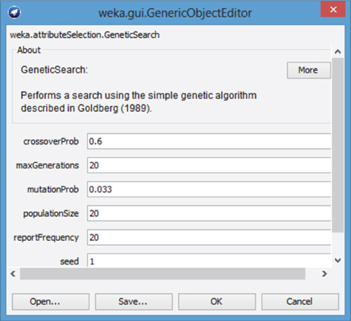
Figure 27.9 Genetic Search dialog.
As specified, the Genetic Search algorithm creates an initial set of 20 chromosomes. An individual chromosome in the initial population may consist of the attribute subset
| 1 | 4 | 6 | 7 | 9 |
where each of the five genes represents an attribute index. For example, the first gene in our example chromosome is the attribute clump_thickness, as represented by its index position = 1. In our configuration, the WrapperSubsetEval evaluation method serves as the fitness function ![]() and calculates a fitness value for each chromosome. WrapperSubsetEval evaluates each of the attribute subsets (chromosomes) according to a specified learning scheme. In the example below we will specify naïve Bayes. This way, the usefulness of a chromosome is determined as a measure of the classification accuracy reported by naïve Bayes. In other words, the chromosomes leading to higher classification accuracy are more relevant and receive a higher fitness score.
and calculates a fitness value for each chromosome. WrapperSubsetEval evaluates each of the attribute subsets (chromosomes) according to a specified learning scheme. In the example below we will specify naïve Bayes. This way, the usefulness of a chromosome is determined as a measure of the classification accuracy reported by naïve Bayes. In other words, the chromosomes leading to higher classification accuracy are more relevant and receive a higher fitness score.
Now, let us apply WEKA's Genetic Search class to our attribute set. To accomplish this task, we first have to specify the evaluator and search options for attribute selection.
- Select the Classify tab.
- Click the Choose button.
- Select Classifiers → Meta → AttributeSelectedClassifier from the navigation hierarchy.
- Now, next to the Choose button, click on the text “AttributeSelectedClassifier …”
The AttributeSelectiedClassifier dialog appears as shown in Figure 27.10, where the default Classifier, Evaluator, and Search methods are displayed. Next, we will override these default options by specifying new classifier, evaluator, and search methods.
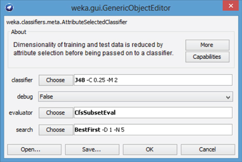
Figure 27.10 AttributeSelectedClassifier dialog.
- Next to evaluator, press the Choose button.
- Select AttributeSelection → WrapperSubsetEval from the navigation hierarchy.
- Now, click on the text “WrapperSubsetEval” next to the evaluator Choose button. The WrapperSubsetEval dialog appears as shown in Figure 27.11. By default, WEKA specifies the ZeroR classifier.
- Press the Choose button, next to classifier.
- Here, select Classifiers → Bayes → Naïve Bayes from the navigation hierarchy.
- Click OK to close the WrapperSubsetEval dialog. The evaluation method for AttributeSelection is now specified.
- On the AttributeSelection dialog, press the Choose button next to search.
- Select AttributeSelection → GeneticSearch from the navigation hierarchy.
- Press OK to close the AttributeSelection dialog.
The evaluator and search methods for attribute selection have been specified. Finally, we specify and execute the classifier.
- Press the Choose button next to classifier.
- Select Classifiers → Bayes → Naïve Bayes.
- Press OK.
- Now, under Test options, specify Use training set
- Click Start
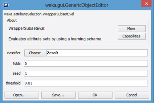
Figure 27.11 WrapperSubsetEval dialog.
WEKA displays modeling results in the Explorer Panel. In particular, under Attributes, notice the list now shows seven predictor attributes, as shown in Table 27.7. That is, the two attributes single_cell_size and mitoses have been removed from the attribute list.
Table 27.7 Attributes selected by the attribute selection method
Selected attributes: |
1,2,3,4,6,7,8 : 7clump_thicknessuniform_cell_sizeuniform_cell_shapemarg_adhesionbare_nucleibland_chromatinnormal_nucleoli |
Naïve Bayes reports 96.93% (662/683) classification accuracy, which indicates the second model outperforms the first model by almost 0.05% (96.93% vs 96.34%). In this example, classification accuracy has increased where only seven of the nine attributes are specified as input. Although these results do not show a dramatic improvement in accuracy, this simple example has demonstrated how WEKA's Genetic Search algorithm can be included as part of an attribute selection approach.
By default, the Genetic Search method specifies default options report frequency = 20 and maxgenerations = 20, which cause WEKA to report population characteristics for the initial and final populations. For example, the initial population characteristics for the 20 chromosomes are shown in Table 27.8.
Table 27.8 Initial population characteristics reported by Genetic Search
Initial population |
||
merit 0.053 0.04978 0.03807 0.05564 0.13177 0.03953 0.0448 0.09048 0.07028 0.04275 0.04187 0.04275 0.08492 0.0612 0.03865 0.03807 0.04275 0.05329 0.05271 0.04275 |
scaled 0.05777 0.06014 0.06873 0.05584 0 0.06765 0.06379 0.03028 0.0451 0.06529 0.06593 0.06529 0.03436 0.05176 0.0683 0.06873 0.06529 0.05756 0.05799 0.06529 |
subset 4 6 7 9 1 2 3 4 7 9 1 2 3 4 6 9 6 7 8 8 2 3 5 6 7 8 2 6 7 5 8 2 1 6 8 9 3 4 5 6 7 8 2 4 6 7 8 4 5 2 4 7 1 2 4 6 7 9 1 3 4 6 9 3 6 7 8 9 2 4 8 1 4 7 8 3 6 7 8 9 |
Here, each subset is a chromosome and merit is the fitness score reported by naïve Bayes, which equals the corresponding classification error rate. For example, consider the chromosome {4, 6, 7, 9} reported in Table 27.8 with merit 0.053; this value corresponds18 to the classification error rate reported by naïve Bayes using fivefold cross-validation when {4, 6, 7, 9} are specified as input.
Also, each chromosome's scaled fitness is reported in the scaled column, where WEKA uses the linear scaling technique to scale the values. By definition, the raw fitness and scaled fitness values have the linear relationship ![]() , where
, where ![]() and
and ![]() are the scaled and raw fitness values, respectively. The constants a and b are chosen where
are the scaled and raw fitness values, respectively. The constants a and b are chosen where ![]() and
and ![]() . The constant
. The constant ![]() represents the expected number of copies of the fittest individual in the population, and for small populations, it is typically set19 to a value in the range of 1.2–2.0.
represents the expected number of copies of the fittest individual in the population, and for small populations, it is typically set19 to a value in the range of 1.2–2.0.
Therefore, by computing the average fitness values presented in Table 27.8, we obtain ![]() and
and ![]() , which agrees with the rule by which the constants a and b are chosen. Because the value for
, which agrees with the rule by which the constants a and b are chosen. Because the value for ![]() is not an option in WEKA, the fitness values from the last two rows from Table 27.8 are selected to solve the simultaneously equations for a and b, according to the relationship
is not an option in WEKA, the fitness values from the last two rows from Table 27.8 are selected to solve the simultaneously equations for a and b, according to the relationship ![]() :
:
Subtracting the second equation from the first, we obtain:

We use the definition ![]() to determine
to determine ![]() . Finally, observe that the fifth row in Table 27.8 has
. Finally, observe that the fifth row in Table 27.8 has ![]() . The raw fitness value of 0.13177 corresponds to the largest classification error in the population produced by chromosome {8}, and as a result,
. The raw fitness value of 0.13177 corresponds to the largest classification error in the population produced by chromosome {8}, and as a result, ![]() is mapped to zero to avoid the possibility of producing negatively scaled fitnesses.
is mapped to zero to avoid the possibility of producing negatively scaled fitnesses.
In this exercise, we have analyzed a simple classification problem where Genetic Search was used to find an attribute subset that improved naïve Bayes classification accuracy, as compared to using the full set of attributes. Although this problem only has nine attributes, there are still ![]() possible attribute subsets that can be input to a classifier. Imagine building a classification model from a set of 100 inputs. Here, there are
possible attribute subsets that can be input to a classifier. Imagine building a classification model from a set of 100 inputs. Here, there are ![]() possible attribute subsets from which to choose. In situations such as these, Genetic Search techniques may prove helpful in determining useful attribute subsets.
possible attribute subsets from which to choose. In situations such as these, Genetic Search techniques may prove helpful in determining useful attribute subsets.
Wisconsin Breast Cancer Database (January 8, 1991). Obtained from the University of Wisconsin Hospitals, Madison from Dr. William H. Wolberg.
R References
- R Core Team. R: A language and environment for statistical computing. Vienna, Austria: R Foundation for Statistical Computing; 2012. ISBN 3-900051-07-0, URL http://www.R-project.org/. Accessed 2014 Sep 30.
- Scrucca, L (2013). GA: a package for genetic algorithms in R. Journal of Statistical Software, 53(4), 1–37. URL http://www.jstatsoft.org/v53/i04/.
Exercises
Clarifying the Concepts
1. Match each of the following genetic algorithm terms with its definition or description.
| Term | Definition |
| a. Selection | One of the candidate solutions to the problem. |
| b. Generation | Scales the chromosome fitness by the standard deviation of the fitnesses, thereby maintaining selection pressure at a constant rate. |
| c. Crowding | The operator that determines which chromosomes will reproduce. |
| d. Crossover | Genes in neighboring loci will often be crossed together, affecting the performance of the genetic algorithm. |
| e. Chromosome | The operator that introduces new information to the genetic pool to protect against premature convergence. |
| f. Positional bias | A feed-forward, completely connected, multilayer network. |
| g. Uniform crossover | A cycle through the genetic algorithm. |
| h. Mutation | One particularly fit chromosome generates too many clones and close copies of itself, thereby reducing population diversity. |
| i. Sigma scaling | The selection condition requiring that the genetic algorithm retains a certain number of the fittest chromosomes from one generation to the next. |
| j. Gene | The operator that performs recombination, creating two new offspring by combining the parents' genes in new ways. |
| k. Elitism | Each gene is randomly assigned to be that of either one parent or the other, with 50% probability. |
| l. Neural Network | A single bit of the candidate solution. |
2. Discuss why the selection operator should be careful to balance fitness with diversity. Describe the dangers of an overemphasis on each.
3. Compare the strengths and weaknesses of using backpropagation and genetic algorithms for optimization in neural networks.
Working with the Data
4. Continue the example in the text, where the fitness is determined by the Normal (16, 4) distribution. Proceed to the end of the third iteration. Suppress mutation, and perform crossover only once, on the second iteration at locus four.
5. Calculate the child vectors for the whole arithmetic crossover example in the text. Use the parents indicated in the section on simple arithmetic crossover, with ![]() . Comment on your results.
. Comment on your results.
Chapter 6 Hands-On Analysis
5. (Extra credit). Write a computer program for a simple genetic algorithm. Implement the example discussed in the text, using the Normal (16, 4) fitness function. Let the crossover rate be 0.6 and the mutation rate be 0.01. Start with the population of all integers 0–31. Generate 25 runs and measure the generation at which the optimal decision of x = 16 is encountered. If you have time, vary the crossover and mutation rates and compare the results.
6. Repeat the procedure using the breast_cancer.arff data set with WEKA by selecting an attribute subset using Genetic Search. This time, however, specify naïve Bayes with use kernel estimator = true for both attribute selection and 10-fold cross-validation. Now, contrast the classification results using the full set of attributes, as compared to the attribute subset selected using Genetic Search. Does classification accuracy improve?