
Chapter 28
Imputation of Missing Data
28.1 Need for Imputation of Missing Data
In this world of big data, the problem of missing data is widespread. It is the rare database that contains no missing values at all. How the analyst deals with the missing data may change the outcome of the analysis, so it is important to learn methods for handling missing data that will not bias the results.
Missing data may arise from any of several different causes. Survey data may be missing because the responder refuses to answer a particular question, or simply skips a question by accident. Experimental observations may be missed due to inclement weather or equipment failure. Data may be lost through a noisy transmission, and so on.
In Chapter 2, we learned three common methods for handling missing data, which are as follows:
- Replace the missing value with some constant, specified by the analyst.
- Replace the missing value with the field mean (for numeric variables) or the mode (for categorical variables).
- Replace the missing values with a value generated at random from the observed distribution of the variable.
We learned that there were problems with each of these methods, which could generate inappropriate data values that would bias our results. For example, in Chapter 2, a value of 400 cu. in. was generated for a vehicle whose cubic inches value was missing. However, this value did not take into account that the vehicle is Japanese, and there is no Japanese-made car in the database that has an engine size of 400 cu. in.
We therefore need data imputation methods that take advantage of the knowledge that the car is Japanese when calculating its missing cubic inches. In data imputation, we ask “What would be the most likely value for this missing value, given all the other attributes for a particular record?” For instance, an American car with 300 cu. in. and 150 hp would probably be expected to have more cylinders than a Japanese car with 100 cu. in. and 90 hp. This is called imputation of missing data. In this chapter, we shall examine methods for imputing missing values for (i) continuous variables and (ii) categorical variables.
28.2 Imputation of Missing Data: Continuous Variables
In Chapter 9, we introduced multiple regression using the cereals data set. It may be worthwhile to take a moment to review the characteristics of the data set by looking back at Chapter 9. We noted that there were four missing data values, which are as follows:
- Potassium content of Almond Delight
- Potassium content of Cream of Wheat
- Carbohydrates and sugars content of Quaker Oatmeal.
Before we use multiple regression to impute these missing values, we must first prepare the data for multiple regression. In particular, the categorical variables must be transformed into 0/1 dummy variables. We did so (not shown) for the variable type, turning it into a flag variable to indicate whether or not the cereal was cold cereal. We then derived a series of dummy variables for the variable manufacturer, with flags for Kellogg's, General Mills, Ralston, and so on.
We begin by using multiple regression to build a good regression model for estimating potassium content. Note that we will be using the variable potassium as the response, and not the original response variable, rating. The idea is to use the set of predictors (apart from potassium) to estimate the potassium content for our Almond Delight cereal. Thus, all the original predictors (minus potassium) represent the predictors, and potassium represents the response variable, for our regression model for imputing potassium content. Do not include the original response variable rating as a predictor for the imputation.
Because not all variables will be significant for predicting potassium, we apply the stepwise variable selection method of multiple regression. In stepwise regression,1 the regression model begins with no predictors, then the most significant predictor is entered into the model, followed by the next most significant predictor. At each stage, each predictor is tested whether it is still significant. The procedure continues until all significant predictors have been entered into the model, and no further predictors have been dropped. The resulting model is usually a good regression model, although it is not guaranteed to be the global optimum.
Figure 28.1 shows the multiple regression results for the model chosen by the stepwise variable selection procedure. The regression equation is:


Figure 28.1 Multiple regression results for imputation of missing potassium values. (The predicted values section of this output is for Almond Delight only.)
To estimate the potassium content for Almond Delight, we plug in Almond Delight's values for the predictors in the regression equation:

That is, the estimated potassium in Almond Delight is 77.9672 mg. This, then, is our imputed value for Almond Delight's missing potassium value: 77.9672 mg.
We may use the same regression equation to estimate the potassium content for Cream of Wheat, plugging in Cream of Wheat's values for the predictors in the regression equation:

The imputed value for Cream of Wheat's missing potassium value is 67.108 mg.
Next, we turn to imputing the missing values for the carbohydrates and sugars content of Quaker Oatmeal. A challenge here is that two predictors have missing values for Quaker Oatmeal. For example, if we build our regression model to impute carbohydrates, and the model requires information for sugars, what value do we use for Quaker Oats sugars, as it is missing? Using the mean or other such ad hoc substitute is unsavory, for the reasons mentioned earlier. Therefore, we will use the following approach:
- Step 1. Build a regression model to impute carbohydrates; do not include sugars as a predictor.
- Step 2. Construct a regression model to impute sugars, using the carbohydrates value found in step 1.
Thus, the values from steps 1 and 2 will represent our imputed values for sugars and carbohydrates. Note that we will include the earlier imputed values for potassium.
Step 1: The stepwise regression model for imputing carbohydrates, based on all the predictors except sugars, is as follows (to save space, the computer output is not shown):

(Note that sugars is not one of the predictors.) Then the imputed step 1 carbohydrates for Quaker Oats is as follows:

Step 2: We then replace the missing carbohydrates value for Quaker Oats with 11.682 in the data set. The stepwise regression model for imputing sugars is:


We insert 4.572 for the missing sugars value for Quaker Oats in the data set, so that there now remain no missing values in the data set.
Now, ambitious programmers may wish to (i) use the imputed 4.572 g sugars value to impute a more precise value for carbohydrates, (ii) use that more precise value for carbohydrates to go back and obtain a more precise value for sugars, and (iii) repeat steps (i) and (ii) until convergence. However, the estimates obtained using a single application of steps 1 and 2 above usually result in a useful approximation of the missing values.
When there are several variables with many missing values, the above step-by-step procedure may be onerous, without recourse to a recursive programming language. In this case, perform the following:
- Step 1: Impute the values of the variable with the fewest missing values. Use only the variables with no missing values as predictors. If no such predictors are available, use the set of predictors with the fewest missing values (apart from the variable you are predicting, of course).
- Step 2: Impute the values of the variable with the next fewest missing values, using similar predictors as used in step 1.
- Step 3: Repeat step 2 until all missing values have been imputed.
28.3 Standard Error of the Imputation
Clients may wish to have an idea of the precision of an imputed value. When estimating or imputing anything, analysts should try to provide a measure of the precision of their estimate or imputation. In this case, the standard error of the imputation2 is used. The formula for the simple linear regression case is:
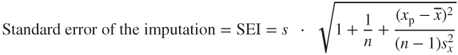
where s is the standard error of the estimate for the regression, ![]() is the value of the known predictor for the particular record,
is the value of the known predictor for the particular record, ![]() represents the mean value of the predictor across all records, and
represents the mean value of the predictor across all records, and ![]() represents the variance of the predictor values.
represents the variance of the predictor values.
For multiple regression (as used here), the formula for SEI is more complex and is best left to the software. Minitab reports SEI as “SE Fit.” In Figure 28.1, where we were imputing Almond Delight's missing potassium value, the standard error of the imputation is SEI = SE Fit = 4.41 mg. This is interpreted as meaning that, in repeated samples of Almond Delight cereal, the typical prediction error for imputing potassium, using the predictors in Figure 28.1, is 1.04 mg.
28.4 Imputation of Missing Data: Categorical Variables
One may use any classification algorithm to impute the missing values of categorical variables. We will illustrate using CART (classification and regression trees, Chapter 8). The data file classifyrisk is a small data file containing 6 fields and 246 records. The categorical predictors are maritalstatus and mortgage; the continuous predictors are income, age, and number of loans. The target is risk, a dichotomous field with values good risk and bad loss. The data file classifyrisk_missing contains a missing value for the marital status of record number 19.
To impute this missing value, we apply CART, with maritalstatus as the target field, and the other predictors as the predictors for the CART model. Z-score standardization is carried out on the continuous variables. The resulting CART model is shown in Figure 28.2.

Figure 28.2 CART model for imputing the missing value of maritalstatus.
Record 19 represents a customer who has the following field values: loans = 1, mortgage = y, age_Z = 1.450, income_Z = 1.498, thus representing a customer who is older than average, with higher income than average, with a mortgage and one other loan. The root node split is on loans; we follow the branch down “loans in [0 1].” The next split checks whether income_Z is greater than 0.812. We follow the branch down “income_Z > 0.812,” which ends at a leaf node containing 30 records, 96.7% of which have a marital status of married. Thus, our imputed value for the marital status of record 19 is married, with a confidence level of 96.7%.
28.5 Handling Patterns in Missingness
The analyst should remain aware that imputation of missing data represents replacement. The data value is now no longer missing; rather, its “missingness” has been replaced with an imputed data value. However, there may be information in the pattern of that missingness, information that will be wasted unless some indicator is provided to the algorithm indicating that this data value had been missing. For example, suppose a study is being made of the effect of a new fertility drug on premenopausal women, and the variable age has some missing values. It is possible that there is a correlation between the age of the subject and the likelihood that the subject declined to give their age. Thus, it may happen that the missing values for age are more likely to occur for greater values of age. Because greater age is associated with infertility, the analyst must account for this possible correlation, by flagging which cases have had their missing ages imputed.
One method to account for patterns in missingness is simply to construct a flag variable, as follows:
Add age_missing to the model, and interpret its effect. For example, in a regression model, perhaps the age_missing dummy variable has a negative regression coefficient, with a very small p-value, indicating significance. This would indicate that indeed there is a pattern in the missingness, namely that the effect size of the fertility drug for those cases whose age value was missing tended to be smaller (or more negative). The flag variable could also be used for classification models, such as CART or C4.5.
Another method for dealing with missing data is to reduce the weight that the case wields in the analysis. This does not account for the patterns in missingness, but rather represents a compromise between no indication of missingness and completely omitting the record. For example, suppose a data set has 10 predictors, and Record 001 has one predictor value missing. Then this missing value could be imputed, and Record 001 assigned a weight, say, of 0.90. Then Record 002, with 2 of 10 field values missing, would be assigned a weight of 0.80. The specific weights assigned depend on the particular data domain and research question of interest. The algorithms would then reduce the amount of influence the records with missing data have on the analysis, proportional to how many fields are missing.
Reference
The classic text on missing data is:
- Little R, Rubin D. Statistical Analysis with Missing Data. second ed. Wiley; 2002.
R References
- Milborrow S. (2012). rpart.plot: Plot rpart models. An enhanced version of plot.rpart. R package version 1.4-3. http://CRAN.R-project.org/package=rpart.plot.
- R Core Team. R: A language and environment for statistical computing. Vienna, Austria: R Foundation for Statistical Computing; 2012. ISBN 3-900051-07-0, URL http://www.R-project.org/. Accessed 2014 Sep 30.
- Therneau T, Atkinson B, and Ripley B (2013). rpart: Recursive Partitioning. R package version 4.1-3. http://CRAN.R-project.org/package=rpart.
Exercises
1. Why do we need to impute missing data?
2. When imputing a continuous variable, explain what we use for the set of predictors, and for the target variable.
3. When imputing a missing value, do we include the original target variable as one of the predictor variables for the data imputation model? Why or why not?
4. Describe what we should do if there are many variables with many missing values.
5. On your own, think of a data set where a potential pattern in missingness would represent good information.
6. State two methods for handling patterns in missingness.
Hands-On Analysis
Use the cereals data set for Exercises 7–12. Report the standard error of each imputation.
7. Impute the potassium content of Almond Delight using multiple regression.
8. Impute the potassium content of Cream of Wheat.
9. Impute the carbohydrates value of Quaker Oatmeal.
10. Impute the sugars value of Quaker Oatmeal.
11. Insert the value obtained in Exercise 10 for the sugars value of Quaker Oatmeal, and impute the carbohydrates value of Quaker Oatmeal.
12. Compare the standard errors for the imputations obtained in Exercises 9 and 11. Explain what you find.
13. Open the ClassifyRisk_Missing data set. Impute the missing value for marital status.
Use the ClassifyRisk_Missing2 data set for Exercises 14–15.
14. Impute all missing values in the data set. Explain the ordering that you are using.
15. Report the standard errors (for continuous values) or confidence levels (for categorical values) for your imputations in Exercise 14.