
Chapter 29
Case Study, Part 1: Business Understanding, Data Preparation, and EDA
In Chapter 29–31 we shall bring together much of what we have learned in this book in a detailed Case Study: Predicting Response to Direct-Mail Marketing. We follow the here in Chapter 29, we (i) enunciate our objectives in the Business Understanding Phase, (ii) get a feel for the data set in Part 1 of the Data Understanding Phase, prepare our data in the Data Preparation Phase, and extract some useful information in Part 2 of the Data Understanding Phase: exploratory data analysis (EDA). Then, in Chapter 30, we learn about possible segments in the customer database using clustering analysis and we investigate relationships among the predictors using principal components analysis. Finally, in Chapter 31, we apply the rich assortment of classification techniques at our disposal in the Modeling Phase, and make recommendations on which models to move forward with in the Evaluation Phase.
29.1 Cross-Industry Standard Practice for Data Mining
The Case Study in Chapter 29–31 will be carried out using the cross-industry standard process for data mining (CRISP-DM). According to CRISP-DM, a given data mining project has a life cycle consisting of six phases, as illustrated in Figure 29.1. The details of CRISP-DM are discussed in Chapter 1; here, we but recapitulate the outline of the process.
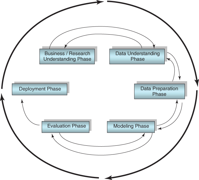
Figure 29.1 CRISP-DM is an iterative, adaptive process.
In practice, the data preparation phase often precedes or is interleaved with the data understanding (EDA) phase, as one may wish to clean up the data before trying to extract information from it. In this chapter, we approach these phases as follows:
29.2 Business Understanding Phase
In the business understanding phase, managers and analysts need to be crystal clear on communicating what the primary objectives of the project are. It often happens that lack of communication/understanding of the primary objectives leads analysts to fashion fine solutions to the wrong problems, like climbing to the top of the ladder, only to find that it is leaning against the wrong wall. To avoid this, a statement of the primary and secondary objectives of the analysis should be agreed upon, by both managers and analysts.
In this detailed Case Study, we are acting as analysts for a retail clothing store chain. The clothing_store data set1 represents actual data provided by a clothing store chain in New England. Data were collected on 51 fields for 28,799 customers. More information about the data set is provided in the Data Understanding Phase below. Here follows the statement of the primary and secondary objectives of the analysis.
For this Case Study, our data mining task is a classification problem. We are to classify which customers will respond to a direct-mail marketing promotion, based on information collected about the customers. However, it will not be sufficient just to derive the classifier with the most accurate predictions. The analyst needs to consider how the classification problem fits into the client's business goals. As we said, for the clothing store, the primary objective is to maximize profits. Therefore, the goal of our classification model should also be to maximize profits, rather than simply to report impressive values for model accuracy, sensitivity, and specificity. To maximize profit, data-driven misclassification costs will be derived and applied.
The specification of data-driven misclassification costs may be considered to belong to the business understanding phase. However, as we will not use the resulting cost matrix until the modeling phase, the derivation of these misclassification costs is postponed until the beginning of the modeling phase (see Chapter 30).
The secondary objective is to develop a better understanding of our customer database using market segment profiles. Specifically, we shall seek to uncover interesting clusters and principal components in our clientele, and, using profiles of these clusters and components, learn more about the different types of customers we have.
29.3 Data Understanding Phase, Part 1: Getting a Feel for the Data Set
In the data understanding phase, we become more familiar with the data set using EDA, graphical and descriptive statistical methods for learning about data. The Clothing_store_training_test data set contains information about 28,799 customers, on the following 51 fields:
- Customer ID: unique, encrypted customer identification
- Zip code
- Number of purchase visits
- Total net sales
- Average amount spent per visit
- Amount spent at each of four different franchises (four variables)
- Amount spent in the past month, the past 3 months, and the past 6 months
- Amount spent the same period last year (SPLY)
- Gross margin percentage
- Number of marketing promotions on file
- Number of days the customer has been on file
- Number of days between purchases
- Markdown percentage on customer purchases
- Number of different product classes purchased
- Number of coupons used by the customer
- Total number of individual items purchased by the customer
- Number of stores the customer shopped at
- Number of promotions mailed in the past year
- Number of promotions responded to in the past year
- Promotion response rate for the past year
- Product uniformity (low score = diverse spending patterns)
- Lifetime average time between visits
- Microvision® Lifestyle Cluster Type
- Percent of returns
- Flag: credit card user
- Flag: valid phone number on file
- Flag: web shopper
- Fifteen variables providing the proportions spent by the customer on specific classes of clothing, including sweaters, knit tops, knit dresses, blouses, jackets, career pants, casual pants, shirts, dresses, suits, outerwear, jewelry, fashion, legwear, and the collectibles line. Also, a variable showing the brand of choice (encrypted).
- Target variable: response to promotion
Assume that these data are based on a direct-mail marketing campaign conducted last year. We shall use this information to develop classification models for this year's marketing campaign.
It is never a bad idea when beginning a new project to take a quick look at the actual data values. Here, Figure 29.2 shows some of the data values for the first 20 records for the first handful of fields.

Figure 29.2 A quick look at the data.
The ID field uniquely identifies each customer (not transaction) in the data set. Looking at the zip code field we immediately spot a problem. American zip codes have five digits; why do these have only four digits? Actually, this is a common problem with zip codes located in New England, which have zero as their initial digit. Somewhere along the line, the zip code field was set to a numeric variable, for which initial zeroes are omitted. We need to replace these initial zeros; one way to perform this is to derive a new zip code field with the following instruction:
where the “><” notation represents “concatenate.” For example, the zip code for the first record in Figure 29.2, “1001,” should really be “01001,” the zip code for Agawam, Massachusetts.
The brand field is using digits to represent a categorical field. This is a potential minefield that may confuse downstream modeling algorithms. The field should be repopulated with letter values rather than numbers. Similarly, the credit card flag field uses 0/1 values, which certain algorithms may incorrectly try to apply operations to that should be reserved for continuous values (e.g., principal components analysis). Therefore, the analyst should be careful with fields like these, and may prefer to substitute F/T values for the 0/1 values. However, 0/1 values for a flag variable are useful as indicator variable predictors in regression and logistic regression. No other major problems leap out at us from Figure 29.2. Note that PSWEATERSraw represents a proportion, but may have been expressed as a percentage instead.
Figure 29.3 shows us an overview of some of the continuous predictors, including a histogram with an overlay of the response (dark = positive response), and some summary statistics. We note immediately that some of the predictors are quite skewed, and will benefit from transformations (discussed below). We may even get a hint of some EDA-flavored results: Responders seem to favor greater days on file and lower average days between purchases.

Figure 29.3 Overview of some of the continuous predictors.
Analysts should never fail to account for missing data. As we discussed in earlier chapters, neglecting to account for missing data, or accounting for missing data in an inappropriate manner, can have deleterious effects on model efficacy. Thankfully, Figure 29.4 indicates that here are no missing values in our data.

Figure 29.4 All fields and records are 100% complete: no missing data.
Next, what is the overall proportion of responders to the direct-mail marketing promotion? Figure 29.5 shows that only 4762 of the 28,799 customers, or 16.54%, responded to last year's marketing campaign (1 indicates response, 0 indicates nonresponse.) As the proportion of responders is so small, we may decide to apply balancing to the data before modeling.
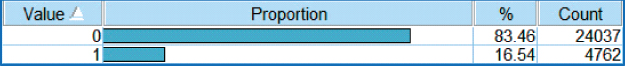
Figure 29.5 Most customers are nonresponders.
One of the variables, the Microvision Lifestyle Cluster Type, contains the market segmentation category for each customer, as defined by Nielsen Claritas. There are 50 segmentation categories, labeled 1–50; the distribution of the most prevalent 18 cluster types over the customer database is given in Figure 29.6.

Figure 29.6 The 20 most prevalent Microvision® Lifestyle Cluster Types.
The six most common lifestyle cluster types in our data set are:
- Cluster 10. Home Sweet Home. Families, medium-high income and education, managers/professionals, technical/sales.
- Cluster 1. Upper Crust. Metropolitan families, very high income and education, homeowners, manager/professionals.
- Cluster 4. Mid-Life Success. Families, very high education, high income, managers/professionals, technical/sales.
- Cluster 16. Country Home Families. Large families, rural areas, medium education, medium income, precision/crafts.
- Cluster 8. Movers and Shakers. Singles, couples, students and recent graduates, high education and income, managers/professionals, technical/sales.
- Cluster 15. Great Beginnings. Young, singles and couples, medium-high education, medium income, some renters, managers/professionals, technical/ sales.
Overall, the clothing store seems to attract a prosperous clientele with fairly high income and education. Cluster 1, Upper Crust, represents the wealthiest of the 50 cluster types, and is the second most prevalent category among our customers. Unfortunately, however, the Microvision variable is more useful for customer description than for modeling, as its values do not help us discern between responders and nonresponders (not shown.) Now, normally, our policy is to retain variables for the modeling stage, even if they do not look significant at the EDA stage. However, because the Microvision variable contains so many different values, its inclusion in certain models (such as logistic regression) can degrade model performance. Thus, we will omit this variable from our modeling.
29.4 Data Preparation Phase
Now that we have a feel for the data set, we turn to the important task of preparing the data for analysis. There are several issues, starting with the unusual issue of negative amounts spent.
29.4.1 Negative Amounts Spent?
For many of the amounts-spent fields and the proportions-spent fields, some of the customers have negative values for the amount or proportion of money spent. See Figure 29.7, where the minimum values for a selection of these variables are negative. How can this be? Now, the data were collected within a particular time period, which is unspecified, perhaps a month or a quarter. It is possible for a customer to have bought some clothing in a prior period, and returned the purchased clothing in the time period from which the data are collected. If this customer also did not make any major purchases during the time period of interest, then the net sales for this customer would be negative.
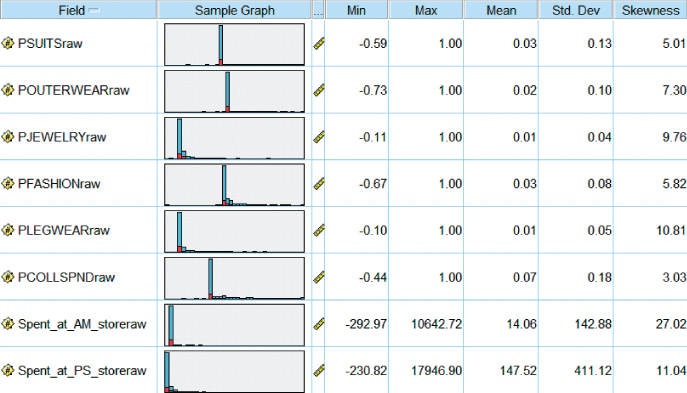
Figure 29.7 The Min values indicate negative amounts spent. How can this be? What should we do about it?
These negative amounts and proportions represent a problem in two ways. First, if we are to apply a transformation, such as the natural log or square root transformation, then we would prefer to be dealing with nonnegative values. Second, if the customers with negative amount spent are more likely than those with zero amount spent to respond to the direct-mail solicitation, then our models may be confused by this, incorrectly expecting the negatives to not respond.
Now, we have a range of options, for how to deal with these negative values.
- Option 1: Treat them as data-entry errors, and either delete the relevant records or apply imputation of missing data.
- Option 2: Leave them as they are.
- Option 3: Change the negative values to zero values.
- Option 4: Take the absolute value of the negative values.
To help us decide how to handle the negative amounts spent problem, let us compare the response rate of these negatives to two other types of customers, those with zero amount spent, and those with positive amount spent. Figure 29.8 shows that 21.57% of those with negative amount spent at the PS store responded positively, compared to 22.19% of those with positive amount spent, and 11.98% of those with zero amount spent. Thus, the customers with negative amount spent have a similar response rate to those with a positive amount spent, both of which are nearly double the response rate of those with zero amount spent. We therefore proceed to take the absolute value of all fields with negative amounts spent or negative proportions spent.
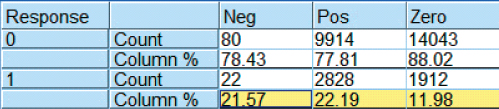
Figure 29.8 Those with negative amount spent have a similar response rate to those with positive amount spent.
Moving to other variables, we turn to the customer ID. As this field is unique to every customer, and is encrypted, it can contain no information that is helpful for our task of predicting which customers are most likely to respond to the direct-mail marketing promotion. It should therefore be omitted from any analytic models. However, the customer ID field should be retained, for housekeeping tasks such as sorting. The zip code can potentially contain information useful in this task. Zip codes, although ostensibly numeric, actually represent a categorization of the client database by geographic locality. However, for the present problem, we set this field aside and concentrate on the remaining variables.
29.4.2 Transformations to Achieve Normality or Symmetry
Most of the numeric fields are right-skewed. For example, Figure 29.9 shows the distribution of product uniformity, a variable which takes large values for customers who purchase only a few different classes of clothes (e.g., blouses, legwear, pants), and small values for customers who purchase many different classes of clothes. Later we shall see that high product uniformity is associated with low probability of responding to the promotion. Figure 29.9 is right-skewed, with most customers having a relatively low product uniformity measure, while fewer customers have larger values. The customers with large values for product uniformity tend to buy only one or two classes of clothes. Note that there are spikes at 100 and at 50; these probably result from how product uniformity is calculated (details not available). It is possible that these spikes contain customers exhibiting specific behaviors, in which case the analyst could derive flag variables to investigate. However, as our time and space are limited, we must move on.
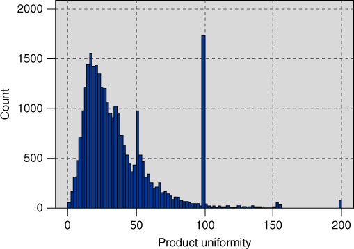
Figure 29.9 Most of the numeric fields are right-skewed, such as product uniformity.
Many data mining methods and models, such as principal components analysis and logistic regression, function best when the variables are normally distributed, or, failing that, at least when they are symmetric. Therefore, we apply transformations to all of the numerical variables that require it, in order to induce approximate normality or symmetry. The analyst may choose from the transformations indicated in Chapter 8, such as the natural log (ln) transformation, the square root transformation, a Box–Cox transformation, or a power transformation from the ladder of reexpressions. For our variables that contained only positive values, we applied the natural log transformation. However, for the variables which contained zero values as well as positive values, we applied the square root transformation, as ![]() is undefined for
is undefined for ![]() .
.
Figure 29.10 shows the distribution of product uniformity, after the natural log transformation. Although perfect normality is not obtained, the result is nevertheless much less skewed than the raw data distribution, allowing for smoother application of several data mining methods and models. Sadly, the spikes remain.
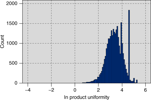
Figure 29.10 Distribution of ln product uniformity is less skewed, although the spikes remain.
Recall that the data set includes 15 variables providing the percentages spent by the customer on specific classes of clothing, including sweaters, knit tops, knit dresses, blouses, and so on. Figure 29.11 shows the distribution of the percentage spent on blouses. We see a spike at zero, along with the usual right-skewness, which calls for a transformation. The square root transformation is applied, with results shown in Figure 29.12. Note that the spike at zero remains, while the remainder of the data appear nicely symmetric.
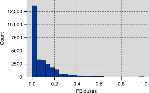
Figure 29.11 Distribution of the percentage spent on blouses.
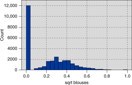
Figure 29.12 Distribution of sqrt percentage spent on blouses.
The dichotomous character of Figure 29.12 motivates us to derive a flag variable for all blouse purchasers. Figure 29.13 shows the distribution of this flag variable, with about 58% of customers having purchased a blouse at one time or another. Flag variables were also constructed for the other 14 clothing percentage variables.

Figure 29.13 Distribution of blouse purchasers flag variable.
29.4.3 Standardization
When there are large differences in variability among the numerical variables, the data analyst needs to apply standardization. The transformations already applied do help in part to reduce the difference in variability among the variables, but substantial differences still exist. For example, the standard deviation for the variable sqrt spending in the last 6 months is 10.03, while the standard deviation for the variable sqrt # coupons used is 0.73. To avoid the greater variability of the variable sqrt spending in the last 6 months overwhelming the variable sqrt # coupons used, the numeric fields should be normalized or standardized. Here, we choose to standardize the numeric fields, so that they all have a mean of zero and a standard deviation of one. For each variable, this is done by subtracting the mean of the variable, and dividing by the standard deviation, to arrive at the z-score. In this analysis, the resulting variable names are prefixed with a “Z” (e.g., z sqrt # coupons used). Other normalization techniques, such as min–max normalization, may be substituted for z-score standardization if desired.
29.4.4 Deriving New Variables
The creation of flag variables for blouse sales and the other item category sales represents deriving new variables, in order to provide greater insight into customer behavior, and hopefully to increase model performance. Further flag variables are constructed as follows. Figure 29.14 shows the histogram of the variable z sqrt spending last 1 month. Note the spike which represents the majority of customers who have not spent any money at the store in the past month. For this reason, flag (indicator) variables were constructed for spending last 1 month, as well as the following variables:
- Spending at the AM store (one of the four franchises), to indicate which customers spent money at this particular store.
- Spending at the PS store
- Spending at the AX store.
- Spending in the last 3 months.
- Spending in the last 6 months.
- Spending in the SPLY.
- Returns, to indicate which customers have ever returned merchandise.
- Response rate, to indicate which customers have ever responded to a marketing promotion before.
- Markdown, to indicate which customers have purchased merchandise which has been marked down.
- No flag is created for spending at the CC store, as all records in the database indicate non-zero amounts spent.

Figure 29.14 Histogram of Z sqrt spending last 1 month motivates us to create a flag variable to indicate which customers spent money in the past month.
The data preparation phase offers the data miner the opportunity to clarify relationships between variables, and to derive new variables that may be useful for the analysis. For example, consider the following three variables:
- Amount spent (by customer) in the last month.
- Amount spent in the last 3 months.
- Amount spent in the last 6 months.
Clearly, the amount spent by the customer in the last month is also contained in the other two variables, the amount spent in the last 3 months and the last 6 months. Therefore, the amount spent in the last month is getting triple-counted. Now, the analyst may not wish for this most recent amount to be so heavily weighted. For example, in time-series models, the more recent measurements are the most heavily weighted. In this case, however, we prefer not to triple-count the most recent month, and must therefore derive two new variables, as shown in Table 29.1.
Table 29.1 New derived spending variables
| Derived Variable | Formula |
| Amount spent in previous months 2 and 3 | Amount spent in last 3 months–amount spent in last 1 month |
| Amount spent in previous months 4–6 | Amount spent in last 6 months–amount spent in last 3 months |
By “amount spent in previous months 2 and 3,” we mean the amount spent in the period 90 to 30 days previous. We shall thus use the following three variables:
- Amount spent in the last month.
- Amount spent in previous months 2 and 3.
- Amount spent in previous months 4, 5, and 6.
And we shall omit the following variables:
- Amount spent in the last 3 months, and
- Amount spent in the last 6 months.
Note that, even with these derived variables, the most recent month's spending may still be considered to be weighted more heavily than any of the other months' spending. This is because the most recent month's spending has its own variable, while the previous 2 and 3 months spending have to share a variable, as do the previous 4, 5, and 6 months spending. Of course, all derived variables should be transformed as needed, and standardized.
The raw data set may have its own derived variables already defined. Consider the following variables:
- Number of purchase visits.
- Total net sales.
- Average amount spent per visit.
The average amount spent per visit represents the ratio:
As the relationship among these variables is functionally defined, it may turn out that the derived variable is strongly correlated with the other variables. The analyst should check this. For example, Figure 29.15 shows that there is strong correlation2 among the variables z ln total net sales, z ln ave spending per visit, and z ln total net sales. This strong correlation shall bear watching; we shall return to this below. By the way, the correlation coefficients between the raw variables should be the same as the correlation coefficients obtained by the Z-scores of those variables.
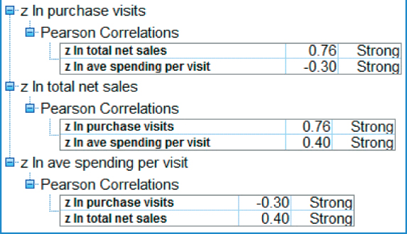
Figure 29.15 Check to make sure the derived variable is not correlated with the original variables.
29.5 Data Understanding Phase, Part 2: Exploratory Data Analysis
Having wrapped up our data preparation, we turn again to the Data Understanding Phase, this time to perform EDA. Recall that EDA allows the analyst to delve into the data set, examine the interrelationships among the variables, identify interesting subsets of observations, and develop an initial idea of possible associations among the predictors, as well as between the predictors and the target variable. And all of this is accomplished without worrying about fulfilling the assumptions required for modeling methods such as regression.
29.5.1 Exploring the Relationships between the Predictors and the Response
We shall return to the correlation issue later, but first we would like to investigate the variable-by-variable association between the predictors and the target variable, response to the marketing promotion. Ideally, the analyst should examine graphs and statistics for every predictor variable, especially with respect to the relationship with the response. However, the huge data sets prevalent in most data mining applications make this a daunting task. Therefore, we would like to have some way to examine the most useful predictors in an exploratory framework.
Of course, choosing the most useful variables is a modeling task, which lies downstream of our present phase, the EDA-flavored data understanding phase. However, a very rough tool for choosing some useful variables to examine at this early phase is correlation. That is, examine the correlation coefficients for each predictor with the response, and select for further examination those variables which have the largest absolute correlations. The analyst should of course be aware that this is simply a rough EDA tool, and linear correlation with a 0–1 response variable is not appropriate for inference or modeling at this stage. Nevertheless, this method can be useful for paring down the number of variables that would be helpful to examine at the EDA stage. Table 29.2 lists the top three predictors with the highest absolute correlation with the target variable, response.
Table 29.2 Variables with largest absolute correlation with the target variable, response
| Variable | Correlation Coefficient | Relationship |
| z ln Lifetime ave time between visits | −0.43 | Negative |
| z ln Purchase visits | 0.40 | Positive |
| z ln # Individual items purchased | 0.37 | Positive |
We therefore examine the relationship between these selected predictors, and the response variable. First, Figure 29.16 shows a histogram of Z ln Lifetime Average Time Between Visits, with an overlay of Response (0 = no response to the promotion). It appears that records at the upper end of the distribution have lower response rates. In order to make the interpretation of overlay results more clearly, we turn to a normalized histogram, where each bin has the same height, shown in Figure 29.17.

Figure 29.16 Histogram of z ln lifetime average time between visits with response overlay: may be difficult to interpret.

Figure 29.17 Normalized histogram of z ln lifetime average time between visits with response overlay: easier to discern pattern.
Figure 29.17 makes it clear that the rate of response to the marketing promotion decreases as the lifetime average time between visits increases. This makes sense, as customers who visit the store more rarely will presumably be less likely to respond to the promotion. Note that presenting the normalized histogram alone is not sufficient, as it does not provide a feel for the original distribution of the variable. Thus, it is usually recommended to provide both the unnormalized and the normalized histograms.
Figure 29.18 shows the nonnormalized and normalized histograms for z ln purchase visits, illustrating that, as the number of purchase visits increases, the response rate increases as well. This is not surprising, as we might anticipate that the customers who shop at our stores often, purchase many different items, spend a lot of money, and buy a lot of different types of clothes, might be interested in responding to our marketing promotion. Figure 29.19 shows the relationship between z ln # individual items purchased and the response variable. We see that, as the number of individual items purchased increases, the response rate increases as well.
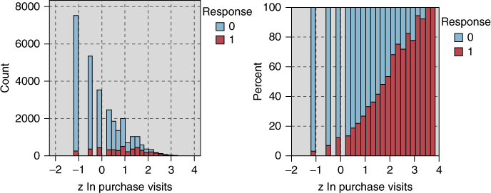
Figure 29.18 As the number of purchase visits increases, the response rate increases as well.

Figure 29.19 As the number of purchase visits increases, so does the response rate.
We might expect that the three variables from Table 29.2 will turn out, in one form or another, to be among the best predictors of promotion response. This is further investigated in the modeling phase.
Next consider Figure 29.20, which shows the normalized histogram of z sqrt percentage spent on blouses, with an overlay of the response variable. Note from Figure 29.20 that, apart from those who spend nothing on blouses (the left-most bin), as the percentage spent on blouses increases, the response rate decreases. This behavior is not restricted to blouses, and is prevalent among all the clothing percentage variables (not shown). What this seems to indicate is that, customers who concentrate on a particular type of clothing, buying only one or two types of clothing (e.g., blouses), tend to have a lower response rate.
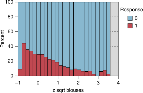
Figure 29.20 z sqrt blouses, with response overlay.
The raw data file contains a variable that measures product uniformity, and, based on the behavior observed in Figure 29.20, we would expect the relationship between product uniformity and response to be negative. This is indeed the case, as shown by the normalized histogram of z ln product uniformity in Figure 29.21. The highest response rate is shown by the customers with the lowest uniformity, that is, the highest diversity of purchasing habits, in other words, customers who purchase many different types of clothing.
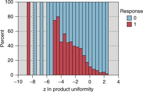
Figure 29.21 As customers concentrate on only one type of clothing, the response rate goes down.
Next, we turn to an examination of the relationship between the response and the many flag variables in the data set. Figure 29.22 provides a directed web graph of the relationship between the response (upper right) and the following indicator variables (counterclockwise from the response): credit card holder, spending months 4, 5, and 6, spending months 2 and 3, spending last 1 month, spending SPLY, returns, response rate, markdown, web buyer, and valid phone number on file. Web graphs are exploratory tools for determining which categorical variables may be of interest for further study.

Figure 29.22 Directed web graph of relationship between the response and several flag variables.
In this graph, only the true values for the various flags are indicated. The darkness and solidity of the line connecting the flag variable with the response is a measure of the association of that variable with the response. In particular, these connections represent percentages of the “true” predictor flag values associated with the “true” value of the response. Therefore, more solid connections represent a greater association with responding to the promotion. Among the most solid connections in Figure 29.22 are the following:
- Web buyer
- Credit card holder
- Spending last 1 month
- Spending SPLY
We therefore examine the normalized distribution of each of these indicator variables, with the response overlay, as shown in Figure 29.23 (positive responses are darker). The counts (and percentages) shown in Figure 29.23 indicate the frequencies (and relative frequencies) of the predictor flag values, and do not represent the proportions shown graphically. To examine these proportions, we turn to the set of contingency tables in Figure 29.24.

Figure 29.23 Higher response rates are associated with (a) web buyers, (b) credit card holders, (c) customers who made a purchase within the past month, and (d) customers who made a purchase in the same period last year.

Figure 29.24 The statistics in these matrices describe the graphics from Figure 29.23.
Consider the highlighted cells in Figure 29.24, which indicate the proportions of customers who have responded to the promotion, conditioned on their flag values. Web buyers (those who have made purchases via the company's web shopping option) are nearly three times as likely to respond compared to those who have not made a purchase via the Web (44.852% vs 15.247%). Credit card holders are also about three times as likely as noncredit card holders (28.066% vs 9.376%) to respond to the promotion. Customers who have made a purchase in the last month are nearly three times as likely to respond to the promotion (33.642% vs 11.981%). Finally, those who made a purchase in the SPLY are twice more likely to respond than those who did not make a purchase during the SPLY (27.312% vs 13.141%). We would therefore expect these flag variables to play some nontrivial role in the model building phase downstream.
29.5.2 Investigating the Correlation Structure among the Predictors
Recall that, depending on the objective of our analysis, we should be aware of the dangers of multicollinearity among the predictor variables. We therefore investigate the pairwise correlation coefficients among the predictors, and note those correlations that are the strongest. Table 29.3 contains a listing of the pairwise correlations that are the strongest in absolute value among the predictors.
Table 29.3 Strongest absolute pairwise correlations among the predictors
| Predictor | Predictor | Correlation |
| z ln Purchase visits | z ln # Different product classes | 0.80 |
| z ln Purchase visits | z ln # Individual items purchased | 0.86 |
| z ln # Promotions on file | z ln # Promotions mailed in last year | 0.89 |
| z ln Total net sales | z ln # Different product classes | 0.86 |
| z ln Total net sales | z ln # Individual items purchased | 0.91 |
| z ln Days between purchase | z ln Lifetime ave time between visits | 0.85 |
| z ln # Different product classes | z ln # Individual items purchased | 0.93 |
Figure 29.25 shows a scatter plot of z ln total net sales versus z ln # individual items purchased, with a response overlay. The strong positive correlation is evident in that, as the number of items purchased increases, the total net sales tends to increase. Of course, such a relationship makes sense, as purchasing more items would presumably tend to result in spending more money. Also, at the high end of both variables (the upper right), responders tend to outnumber nonresponders, while at the lower end (the lower left), the opposite is true.
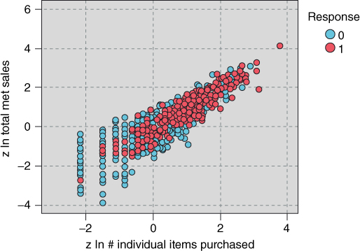
Figure 29.25 Scatter plot of a positive relationship: z ln total net sales versus z ln # individual items purchased, with response overlay.
For an example of a negative relationship, we may turn to Figure 29.26, the scatter plot of z gross margin percentage versus z markdown, with response overlay. The correlation between these variables is −0.77, and so they did not make the list in Table 29.3. In the scatter plot, it is clear that, as markdown increases, the gross margin percentage tends to decrease.

Figure 29.26 Scatter plot of a negative relationship: z gross margin % versus z markdown.
If the number of predictors is large, however, evaluating individual scatter plot may become tedious. This is because, for k predictors, there are kC2 possible two-dimensional scatter plots. For example, for 10 predictors, there are 45 possible scatter plots. It can be more convenient, therefore, to use matrix plots, which provide several scatter plots at one time. Figure 29.27 is an example of a matrix plot for the predictors z ln days between purchases, z ln lifetime ave time betw visits, and z ln # individual items purchased, with an overlay of response. The plots along the diagonal are histograms of the respective predictors. Note the positive relationship between z ln days between purchases and z ln lifetime ave time betw visits (plot in the middle of the left-hand column), which makes sense as customers who have shorter times between visits to the store are likely to have shorter times between purchases at the store. These customers tend toward the lower left of the plot, and indicate a greater response rate than the other customers. Also one may consider the negative relationship between z ln days between purchases and z ln # individual items purchased (plot in the lower left). It makes sense that, as customers wait longer between purchases, they will tend to make a lower overall number of individual items purchased. Also, there is a hint in the upper left of this last graph of a greater response rate, as these are the customers with smaller days between purchases, and higher number of individual items purchased.
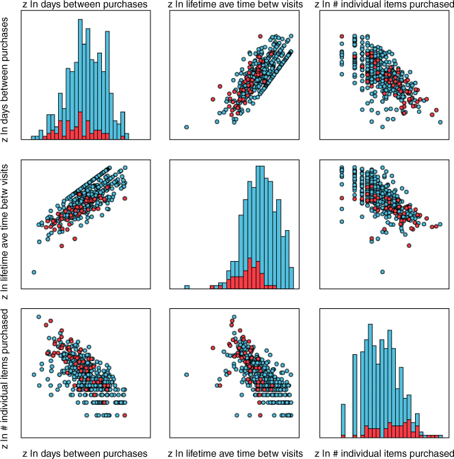
Figure 29.27 Matrix plot of three predictors, showing positive and negative relationships.
A convenient method for examining the relationship between categorical variables and response is a contingency table, (or cross-tabulation), using a function of the response instead of raw cell counts. For example, suppose we are interested in the relationship between response to the promotion and two types of customers: those who have purchased sweaters and those who have made a purchase within the last month. Figure 29.28 contains such a cross-tabulation, with the cells representing the mean value of the target variable (response). As the target represents a dichotomous variable, the means therefore represent proportions.
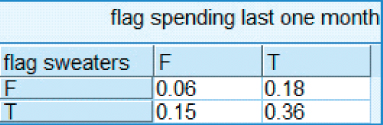
Figure 29.28 Cross-tabulation of spending within the last month versus sweater purchase, with cell values representing promotion response percentages.
Thus, in the cross-tabulation, we see that the customers who have neither bought sweaters nor made a purchase in the last month have only a 0.06 probability of responding to the direct-mail marketing promotion. However, customers who have both bought a sweater and made a purchase in the last month have a 0.36 probability of responding positively to the promotion.
29.5.3 Importance of De-Transforming for Interpretation
We provide an example to illustrate how analysts presenting results to clients and managers should take care to de-transform their statistical results. Figure 29.29 contains a cross-tabulation of web buyers versus credit card users, with the cells containing the mean of z ln purchase visits for the customers in each cell. Note that customers with positive values for both flag variables have the highest means, and customers with negative values for both have the lowest means. This is good information, but limited. We cannot tell from this information, the actual mean number of purchase visits for each cell. In order to find this information, we need to de-transform, which means to take the inverse of the original transformation.
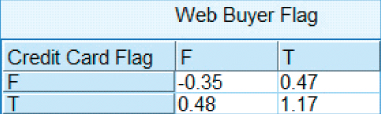
Figure 29.29 Cross-tabulation of web buyers versus credit card users, with cells containing z ln purchase visits.
Thus, to find the mean number of purchase visits for those customers who are both web buyers and credit card users, we need to (i) first apply the inverse Z transformation, and then (ii) apply the inverse ln transformation. The mean number of purchase visits for all customers is ![]() with standard deviation of
with standard deviation of ![]() visits. Apply the inverse Z transformation gives us
visits. Apply the inverse Z transformation gives us
Then, applying the inverse ln transformation, we get:
Thus, the mean number of purchase visits for web buyers who are also credit card users is 9.28 visits. However, the mean number of purchase visits who are neither web buyers not credit card users is
Thus, customers who are both web buyers and credit card holders have more than three times as many purchase visits as customers who are neither web buyers nor credit card holders. These are results that are understandable and actionable by clients and managers.
Here in Chapter 29, we have illustrated how to use EDA to learn more about our customer clientele, which represents part of the secondary objective of our Case Study. Of course, much more could be done along these lines, but space limitations restrict us to the examples above. Next, in Chapter 30, we learn more about our customers through the use of principal components analysis and clustering analysis.