
7.4 Solving Flair Furniture’s LP Problem Using QM for Windows, Excel 2016, and Excel QM
Almost every organization has access to computer programs that are capable of solving enormous LP problems. Although each computer program is slightly different, the approach each takes toward handling LP problems is basically the same. The format of the input data and the level of detail provided in output results may differ from program to program and computer to computer, but once you are experienced in dealing with computerized LP algorithms, you can easily adjust to minor changes.
Using QM for Windows
Let us begin by demonstrating QM for Windows on the Flair Furniture Company problem. To use QM for Windows, select the Linear Programming module. Then specify the number of constraints (other than the nonnegativity constraints, as it is assumed that the variables must be nonnegative), the number of variables, and whether the objective is to be maximized or minimized. For the Flair Furniture Company problem, there are two constraints and two variables. Once these numbers are specified, the input window opens, as shown in Program 7.1A. Then you can enter the coefficients for the objective function and the constraints. Placing the cursor over X1 and X2 and typing new names, such as T and C, will change the variable names. The constraint names can be similarly modified. Program 7.1B shows the QM for Windows screen after the data have been input and before the problem is solved. When you click the Solve button, you get the output shown in Program 7.1C.

Program 7.1A QM for Windows Linear Programming Input Screen

Program 7.1B QM for Windows Data Input for Flair Furniture Problem

Program 7.1C QM for Windows Output and Graph for Flair Furniture Problem
Once the problem has been solved, a graph may be displayed by selecting Window—Graph from the menu bar in QM for Windows. Program 7.1C shows the output for the graphical solution. Notice that in addition to the graph, the corner points and the original problem are shown. Later we return to see additional information related to sensitivity analysis that is provided by QM for Windows.
Using Excel’s Solver Command to Solve LP Problems
Excel 2016 (as well as earlier versions) has an add-in called Solver that can be used to solve linear programs. If this add-in doesn’t appear on the Data tab in Excel 2016, it has not been activated. See Appendix F for details on how to activate it.
Preparing the Spreadsheet For Solver
The spreadsheet must be prepared with data and formulas for certain calculations before Solver can be used. Excel QM can be used to simplify this process (see Appendix F). We will briefly describe the steps, and further discussion and suggestions will be provided when the Flair Furniture example is presented. Here is a summary of the steps to prepare the spreadsheet:
Enter the problem data. The problem data consist of the coefficients of the objective function and the constraints, plus the RHS value for each of the constraints. It is best to organize this in a logical and meaningful way. The coefficients will be used when writing formulas in steps 3 and 4, and the RHS will be entered into Solver.
Designate specific cells for the values of the decision variables. Later, these cell addresses will be input into Solver.
Write a formula to calculate the value of the objective function, using the coefficients for the objective function (from step 1) that you have entered and the cells containing the values of the decision variables (from step 2). Later, this cell address will be input into Solver.
Write a formula to calculate the value of the LHS of each constraint, using the coefficients for the constraints (from step 1) that you have entered and the cells containing the values of the decision variables (from step 2). Later, these cell addresses and the cell addresses for the corresponding RHS values will be input into Solver.
These four steps must be completed in some way with all linear programs in Excel. Additional information may be put into the spreadsheet for clarification purposes. Let’s illustrate these with an example.
Program 7.2A provides the input data for the Flair Furniture example. You should enter the numbers in the cells shown. The words can be any description that you choose. The “” symbols are entered for reference only. They are not specifically used by Excel Solver.
The cells designated for the values of the variables are B4 for T (tables) and C4 for C (chairs). These cell addresses will be entered into Solver in the By Changing Variables Cells box. Solver will change the values in these cells to find the optimal solution. It is sometimes helpful to enter a 1 in each of these to help identify any obvious errors when the formulas for the objective and the constraints are written.
A formula is written in Excel for the objective function (D5), and this is displayed in Program 7.2B. The Sumproduct function is very helpful, although there are other ways to write this. This cell address will be entered into Solver in the Set Objective box.
The hours used in carpentry (the LHS of the carpentry constraint) are calculated with the formula in cell D8, while cell D9 calculates the hours used in painting, as illustrated in Program 7.2B. These cells and the cells containing the RHS values will be used when the constraints are entered into Solver.

Program 7.2A Excel Data Input for Flair Furniture Example

Program 7.2B Formulas for Flair Furniture Example
The problem is now ready for the use of Solver. However, even if the optimal solution is not found, this spreadsheet has benefits. You can enter different values for T and C into cells B4 and C4 just to see how the resource utilization (LHS) and profit change.
Using Solver
To begin using Solver, go to the Data tab in Excel 2016 and click Solver, as shown in Program 7.2D. If Solver does not appear on the Data tab, see Appendix F for instructions on how to activate this add-in. Once you click Solver, the Solver Parameters dialog box opens, as shown in Program 7.2E, and the following inputs should be entered, although the order is not important:

Program 7.2D Starting Solver in Excel 2016
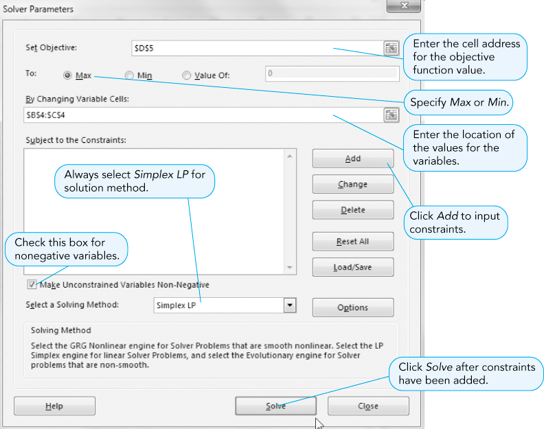
Program 7.2E Solver Parameters Dialog Box
In the Set Objective box, enter the cell address for the total profit (D5).
In the By Changing Variable Cells box, enter the cell addresses for the variable values (B4:C4). Solver will allow the values in these cells to change while searching for the best value in the Set Objective cell reference.
Click Max for a maximization problem and Min for a minimization problem.
Check the box for Make Unconstrained Variables Non-Negative, since the variables T and C must be greater than or equal to zero.
Click the Select Solving Method button and select Simplex LP from the menu that appears.
Click Add to add the constraints. When you do this, the dialog box shown in Program 7.2F appears.
In the Cell Reference box, enter the cell references for the LHS values (D8:D9). Click the button to open the drop-down menu to select which is forconstraints. Then enter the cell references for the RHS values (F8:F9). Since these are all less-than-or-equal-to constraints, they can all be entered at one time by specifying the ranges. If there were other types of constraints, such as constraints, you could click Add after entering these first constraints, and the Add Constraint dialog box would allow you to enter additional constraints. When preparing the spreadsheet for Solver, it is easier if all theconstraints are together and all theconstraints are together. After entering all the constraints, click OK. The Add Constraint dialog box closes, and the Solver Parameters dialog box reopens.
Click Solve on the Solver Parameters dialog box, and the solution is found. The Solver Results dialog box opens and indicates that a solution was found, as shown in Program 7.2G. In situations where there is no feasible solution, this box will indicate this. Additional information may be obtained from the Reports section of this box, as will be seen later. Program 7.2H shows the results of the spreadsheet with the optimal solution.

Program 7.2F Solver Add Constraint Dialog Box

Program 7.2G Solver Results Dialog Box

Program 7.2H Flair Furniture Solution Found by Solver
Using Excel QM
Using the Excel QM add-in can help you easily solve linear programming problems. Not only are all formulas automatically created by Excel QM, but also the spreadsheet is automatically prepared for the use of the Solver add-in. We will illustrate this using the Flair Furniture example.
To begin, from the Excel QM ribbon in Excel 2016, click the Alphabetical menu, and then select Linear, Integer & Mixed Integer Programming from the drop-down menu, as shown in Program 7.3A. The Excel QM Spreadsheet Initialization window opens, and in it, you enter the problem title, the number of variables, and the number of constraints (do not count the nonnegativity constraints). Specify whether the problem is a maximization or minimization problem, and then click OK. When the initialization process is finished, a spreadsheet is prepared for data input, as shown in Program 7.3B. In this worksheet, enter the data in the section labeled Data. Specify the type of constraint (less-than, greater-than, or equal-to), and change the variable names and the constraint names, if desired. You do not have to write any formulas.
Once the data have been entered, from the Data tab, select Solver. The Solver Parameters window opens (refer back to Program 7.2E to see what input is normally required in a typical Solver Parameters window), and you will see that Excel QM has made all the necessary inputs and selections. You do not enter any information, and you simply click Solve to find the solution. The solution is displayed in Program 7.3C.

Program 7.2C Excel Spreadsheet for Flair Furniture Example

Program 7.3A Using Excel QM in Excel 2016 for the Flair Furniture Example

Program 7.3B Excel QM Data Input for the Flair Furniture Example
