
13.2 Monte Carlo Simulation
When a system contains elements that exhibit chance in their behavior, the Monte Carlo method of simulation can be applied.
The basic idea in Monte Carlo simulation is to generate values for the variables making up the model being studied. There are a lot of variables in real-world systems that are probabilistic in nature and that we might want to simulate. A few examples of these variables follow:
Inventory demand on a daily or weekly basis
Lead time for inventory orders to arrive
Times between machine breakdowns
Times between arrivals at a service facility
Service times
Times to complete project activities
Number of employees absent from work each day
Some of these variables, such as the daily demand and the number of employees absent, are discrete and must be integer valued. For example, the daily demand can be 0, 1, 2, 3, and so forth. But daily demand cannot be 4.7362 or any other noninteger value. Other variables, such as those related to time, are continuous and are not required to be integers because time can be any value. When selecting a method to generate values for the random variable, this characteristic of the random variable should be considered. Examples of both will be given in the following sections.
The basis of Monte Carlo simulation is experimentation on the chance (or probabilistic) elements through random sampling. The technique breaks down into five simple steps:
Five Steps of Monte Carlo Simulation
Establishing probability distributions for important input variables
Building a cumulative probability distribution for each variable in step 1
Establishing an interval of random numbers for each variable
Generating random numbers
Simulating a series of trials
We will examine each of these steps and illustrate them with the following example.
Harry’s Auto Tire Example
Harry’s Auto Tire sells all types of tires, but a popular radial tire accounts for a large portion of Harry’s overall sales. Recognizing that inventory costs can be quite significant with this product, Harry wishes to determine a policy for managing this inventory. To see what the demand would look like over a period of time, he wishes to simulate the daily demand for a number of days.
Step 1: Establishing Probability Distributions.
One common way to establish a probability distribution for a given variable is to examine historical outcomes. The probability, or relative frequency, for each possible outcome of a variable is found by dividing the frequency of observation by the total number of observations. The daily demand for radial tires at Harry’s Auto Tire over the past 200 days is shown in Table 13.1. We can convert these data to a probability distribution, if we assume that past demand rates will hold in the future, by dividing each demand frequency by the total demand, 200.
Table 13.1 Historical Daily Demand for Radial Tires at Harry’s Auto Tire and Probability Distribution
| DEMAND FOR TIRES | FREQUENCY (DAYS) | PROBABILITY OF OCCURRENCE |
|---|---|---|
| 0 | 10 | |
| 1 | 20 | |
| 2 | 40 | |
| 3 | 60 | |
| 4 | 40 | |
| 5 | 30 | |
| 200 |
Probability distributions, we should note, need not be based solely on historical observations. Often, managerial estimates based on judgment and experience are used to create a distribution. Sometimes, a sample of sales, machine breakdowns, or service rates is used to create probabilities for those variables. And the distributions themselves can be either empirical, as in Table 13.1, or based on the commonly known normal, binomial, Poisson, or exponential patterns.
Step 2: Building a Cumulative Probability Distribution for Each Variable.
The conversion from a regular probability distribution, such as in the right-hand column of Table 13.1, to a cumulative distribution is an easy job. A cumulative probability is the probability that a variable (demand) will be less than or equal to a particular value. A cumulative distribution lists all of the possible values and the probabilities. In Table 13.2, we see that the cumulative probability for each level of demand is the sum of the number in the probability column (middle column) and the previous cumulative probability (rightmost column). The cumulative probability, graphed in Figure 13.2, is used in step 3 to help assign random numbers.
Step 3: Setting Random Number Intervals.
After we have established a cumulative probability distribution for each variable included in the simulation, we must assign a set of numbers to represent each possible value or outcome. These are referred to as random number intervals. Random numbers are discussed in detail in step 4. Basically, a random number is a series of digits (say, two digits from 01, 02, …, 98, 99, 00) that have been selected by a totally random process.
If there is a 5% chance that demand for a product (such as Harry’s radial tires) is 0 units per day, we want 5% of the random numbers available to correspond to a demand of 0 units. If a total of 100 two-digit numbers is used in the simulation (think of them as being numbered chips in a bowl), we could assign a demand of 0 units to the first five random numbers: 01, 02, 03, 04, and 05.1 Then a simulated demand for 0 units would be created every time one of the numbers 01 to 05 was drawn. If there is also a 10% chance that demand for the same product is 1 unit per day, we could let the next 10 random numbers (06, 07, 08, 09, 10, 11, 12, 13, 14, and 15) represent that demand—and so on for other demand levels.
In general, using the cumulative probability distribution computed and graphed in step 2, we can set the interval of random numbers for each level of demand in a very simple fashion. You will note in Table 13.3 that the interval selected to represent each possible daily demand is very closely related to the cumulative probability on its left. The top end of each interval is always equal to the cumulative probability percentage.
Similarly, we can see in Figure 13.2 and in Table 13.3 that the length of each interval on the right corresponds to the probability of one of each of the possible daily demands. Hence, in assigning random numbers to the daily demand for three radial tires, the range of the random number interval (36 to 65) corresponds exactly to the probability (or proportion) of that outcome. A daily demand for three radial tires occurs 30% of the time. One of the 30 random numbers greater than 35 up to and including 65 is assigned to that event.
Step 4: Generating Random Numbers.
Random numbers may be generated for simulation problems in several ways. If the problem is very large and the process being studied involves thousands of simulation trials, computer programs are available to generate the random numbers needed.
Table 13.2 Cumulative Probabilities for Radial Tires
| DAILY DEMAND | PROBABILITY | CUMULATIVE PROBABILITY |
|---|---|---|
| 0 | 0.05 | 0.05 |
| 1 | 0.10 | 0.15 |
| 2 | 0.20 | 0.35 |
| 3 | 0.30 | 0.65 |
| 4 | 0.20 | 0.85 |
| 5 | 0.15 | 1.00 |

Figure 13.2 Graphical Representation of the Cumulative Probability Distribution for Radial Tires
If the simulation is being done by hand, as in this book, the numbers may be selected spinning a roulette wheel that has 100 slots, by blindly grabbing numbered chips out of a hat, or by any method that allows you to make a random selection.2 The most commonly used means is to choose numbers from a table of random digits such as Table 13.4.
Table 13.4 was itself generated by a computer program. It has the characteristic that every digit or number in it has an equal chance of occurring. In a very large random number table, 10% of digits would be 1s, 10% 2s, 10% 3s, and so on. Because everything is random, we can select numbers from anywhere in the table to use in our simulation procedures in step 5.
Step 5: Simulating the Experiment.
We can simulate outcomes of an experiment by simply selecting random numbers from Table 13.4. Beginning anywhere in the table, we note the interval in Table 13.3 or Figure 13.2 into which each number falls. For example, if the random number chosen is 81 and the interval 66 to 85 represents a daily demand for four tires, we select a demand of four tires.
Table 13.3 Assignment of Random Number Intervals for Harry’s Auto Tire
| DAILY DEMAND | PROBABILITY | CUMULATIVE PROBABILITY | INTERVAL OF RANDOM NUMBERS |
|---|---|---|---|
| 0 | 0.05 | 0.05 | 01 to 05 |
| 1 | 0.10 | 0.15 | 06 to 15 |
| 2 | 0.20 | 0.35 | 16 to 35 |
| 3 | 0.30 | 0.65 | 36 to 65 |
| 4 | 0.20 | 0.85 | 66 to 85 |
| 5 | 0.15 | 1.00 | 86 to 00 |
Table 13.4 Table of Random Numbers
| 52 | 06 | 50 | 88 | 53 | 30 | 10 | 47 | 99 | 37 | 66 | 91 | 35 | 32 | 00 | 84 | 57 | 07 |
| 37 | 63 | 28 | 02 | 74 | 35 | 24 | 03 | 29 | 60 | 74 | 85 | 90 | 73 | 59 | 55 | 17 | 60 |
| 82 | 57 | 68 | 28 | 05 | 94 | 03 | 11 | 27 | 79 | 90 | 87 | 92 | 41 | 09 | 25 | 36 | 77 |
| 69 | 02 | 36 | 49 | 71 | 99 | 32 | 10 | 75 | 21 | 95 | 90 | 94 | 38 | 97 | 71 | 72 | 49 |
| 98 | 94 | 90 | 36 | 06 | 78 | 23 | 67 | 89 | 85 | 29 | 21 | 25 | 73 | 69 | 34 | 85 | 76 |
| 96 | 52 | 62 | 87 | 49 | 56 | 59 | 23 | 78 | 71 | 72 | 90 | 57 | 01 | 98 | 57 | 31 | 95 |
| 33 | 69 | 27 | 21 | 11 | 60 | 95 | 89 | 68 | 48 | 17 | 89 | 34 | 09 | 93 | 50 | 44 | 51 |
| 50 | 33 | 50 | 95 | 13 | 44 | 34 | 62 | 64 | 39 | 55 | 29 | 30 | 64 | 49 | 44 | 30 | 16 |
| 88 | 32 | 18 | 50 | 62 | 57 | 34 | 56 | 62 | 31 | 15 | 40 | 90 | 34 | 51 | 95 | 26 | 14 |
| 90 | 30 | 36 | 24 | 69 | 82 | 51 | 74 | 30 | 35 | 36 | 85 | 01 | 55 | 92 | 64 | 09 | 85 |
| 50 | 48 | 61 | 18 | 85 | 23 | 08 | 54 | 17 | 12 | 80 | 69 | 24 | 84 | 92 | 16 | 49 | 59 |
| 27 | 88 | 21 | 62 | 69 | 64 | 48 | 31 | 12 | 73 | 02 | 68 | 00 | 16 | 16 | 46 | 13 | 85 |
| 45 | 14 | 46 | 32 | 13 | 49 | 66 | 62 | 74 | 41 | 86 | 98 | 92 | 98 | 84 | 54 | 33 | 40 |
| 81 | 02 | 01 | 78 | 82 | 74 | 97 | 37 | 45 | 31 | 94 | 99 | 42 | 49 | 27 | 64 | 89 | 42 |
| 66 | 83 | 14 | 74 | 27 | 76 | 03 | 33 | 11 | 97 | 59 | 81 | 72 | 00 | 64 | 61 | 13 | 52 |
| 74 | 05 | 81 | 82 | 93 | 09 | 96 | 33 | 52 | 78 | 13 | 06 | 28 | 30 | 94 | 23 | 37 | 39 |
| 30 | 34 | 87 | 01 | 74 | 11 | 46 | 82 | 59 | 94 | 25 | 34 | 32 | 23 | 17 | 01 | 58 | 73 |
| 59 | 55 | 72 | 33 | 62 | 13 | 74 | 68 | 22 | 44 | 42 | 09 | 32 | 46 | 71 | 79 | 45 | 89 |
| 67 | 09 | 80 | 98 | 99 | 25 | 77 | 50 | 03 | 32 | 36 | 63 | 65 | 75 | 94 | 19 | 95 | 88 |
| 60 | 77 | 46 | 63 | 71 | 69 | 44 | 22 | 03 | 85 | 14 | 48 | 69 | 13 | 30 | 50 | 33 | 24 |
| 60 | 08 | 19 | 29 | 36 | 72 | 30 | 27 | 50 | 64 | 85 | 72 | 75 | 29 | 87 | 05 | 75 | 01 |
| 80 | 45 | 86 | 99 | 02 | 34 | 87 | 08 | 86 | 84 | 49 | 76 | 24 | 08 | 01 | 86 | 29 | 11 |
| 53 | 84 | 49 | 63 | 26 | 65 | 72 | 84 | 85 | 63 | 26 | 02 | 75 | 26 | 92 | 62 | 40 | 67 |
| 69 | 84 | 12 | 94 | 51 | 36 | 17 | 02 | 15 | 29 | 16 | 52 | 56 | 43 | 26 | 22 | 08 | 62 |
| 37 | 77 | 13 | 10 | 02 | 18 | 31 | 19 | 32 | 85 | 31 | 94 | 81 | 43 | 31 | 58 | 33 | 51 |
| Source: Excerpts from A Million Random Digits with 100,000 Normal Deviates, The Free Press, 1955, © RAND Corporation. Reprinted with permission. | |||||||||||||||||
We now illustrate the concept further by simulating 10 days of demand for radial tires at Harry’s Auto Tire (see Table 13.5). We select the random numbers needed from Table 13.4, starting in the upper left-hand corner and continuing down the first column.
It is interesting to note that the average demand of 3.9 tires in this 10-day simulation differs significantly from the expected daily demand, which we can compute from the data in Table 13.2:
If this simulation were repeated hundreds or thousands of times, it is much more likely that the average simulated demand would be nearly the same as the expected demand.
Naturally, it would be risky to draw any hard and fast conclusions regarding the operation of a firm from only a short simulation. However, this simulation by hand demonstrates the important principles involved. It helps us to understand the process of Monte Carlo simulation that is used in computerized simulation models.
The simulation for Harry’s Auto Tire involved only one variable. The true power of simulation is seen when several random variables are involved and the situation is more complex. In Section 13.4, we see a simulation of an inventory problem in which both the demand and the lead time may vary.
As you might expect, the computer can be a very helpful tool in carrying out the tedious work in larger simulation undertakings. We now demonstrate how QM for Windows and Excel can both be used for simulation.
Using QM for Windows for Simulation
Program 13.1 is a Monte Carlo simulation using the QM for Windows software. Inputs to this model are the possible values for the variable, the number of trials to be generated, and either the associated frequency or the probability for each value. If frequencies are input, QM for Windows will compute the probabilities, as well as the cumulative probability distribution. We see that the expected value (2.95) is computed mathematically, and we can compare the actual sample average (2.87) with this. If another simulation is performed, the sample average may change.
Table 13.5 Ten-Day Simulation of Demand for Radial Tires
| DAY | RANDOM NUMBER | SIMULATED DAILY DEMAND |
|---|---|---|
| 1 | 52 | 3 |
| 2 | 37 | 3 |
| 3 | 82 | 4 |
| 4 | 69 | 4 |
| 5 | 98 | 5 |
| 6 | 96 | 5 |
| 7 | 33 | 2 |
| 8 | 50 | 3 |
| 9 | 88 | 5 |
| 10 | 90 | 5 |
| 10-day demand | ||
| daily demand for tires |

Program 13.1 QM for Windows Output Screen for Simulation of Harry’s Auto Tire Example

Program 13.2 Using Excel 2016 to Simulate Tire Demand for Harry’s Auto Tire Shop
| KEY FORMULAS | |
|---|---|
 Copy H3:I3 to H4:I12
|
 Copy C4:D4 to C5:D8 Copy C4:D4 to C5:D8
|
|
|
 Copy D17:E17 to D18:E21 Copy D17:E17 to D18:E21
|
Simulation with Excel Spreadsheets
The ability to generate random numbers and then “look up” these numbers in a table in order to associate them with a specific event makes spreadsheets excellent tools for conducting simulations. Program 13.2 illustrates an Excel simulation for Harry’s Auto Tire.
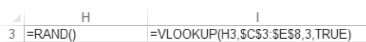
The function is used to generate a random number between 0 and 1. The function looks up the random number in the leftmost column of the defined lookup table It moves downward through this column until it finds a cell that is bigger than the random number. It then goes to the previous row and gets the value from column E of the table.
In Program 13.2, for example, the first random number shown is 0.474807. Excel looked down the left-hand column of the lookup table of Program 13.2 until it found 0.65. From the previous row, it retrieved the value in column E, which is 3. Pressing the F9 function key recalculates the random numbers and the simulation.
The FREQUENCY function in Excel (column C in Program 13.2) is used to tabulate how often a value occurs in a set of data. This is an array function, so special procedures are required to enter it. First, highlight the entire range where this is to be located Then enter the function, as illustrated in cell C16, and press This causes the formula to be entered as an array into all the cells that were highlighted
Many problems exist in which the variable to be simulated is normally distributed and thus is a continuous variable. A function in Excel makes generating normal random numbers very easy, as seen in Program 13.3. The mean is 40 and the standard deviation is 5. The format is
In Program 13.3, the 200 simulated values for the normal random variable are generated in column A.
A chart (cells C3:E19) was developed to show the distribution of the randomly generated numbers.
Excel QM has a simulation module that is very easy to use. When Simulation is selected from the Excel QM menu, an Initialization window opens, and you enter the number of categories and the number of simulation trials you want to run. A spreadsheet will be developed, and you then enter the values and the frequencies, as shown in Program 13.4. The actual random numbers and their associated demand values are also displayed in the output, but they are not shown in Program 13.4.

Program 13.3 Generating Normal Random Numbers in Excel 2016
| KEY FORMULAS | |
|---|---|
|
|
|
|
|
|
