
M8.2 The Assignment Algorithm
The second special-purpose LP algorithm discussed in this module is the assignment method. Each assignment problem has associated with it a table, or matrix. Generally, the rows contain the objects or people we wish to assign, and the columns comprise the tasks or things we want them assigned to. The numbers in the table are the costs associated with each particular assignment.
An assignment problem can be viewed as a transportation problem in which the capacity from each source (or person to be assigned) is 1 and the demand at each destination (or job to be done) is 1. Such a formulation could be solved using the transportation algorithm, but it would have a severe degeneracy problem. However, this type of problem is very easy to solve using the assignment method.
As an illustration of the assignment method, let us consider the case of the Fix-It Shop, which has just received three new rush projects to repair: (1) a radio, (2) a toaster oven, and (3) a broken coffee table. Three repair persons, each with different talents and abilities, are available to do the jobs. The Fix-It Shop owner estimates what it will cost in wages to assign each of the workers to each of the three projects. The costs, which are shown in Table M8.15, differ because the owner believes that each worker will differ in speed and skill on these quite varied jobs.
Table M8.15 Estimated Project Repair Costs for the Fix-It Shop Assignment Problem
| PROJECT | |||
|---|---|---|---|
| PERSON | 1 | 2 | 3 |
| Adams | $11 | $14 | $6 |
| Brown | 8 | 10 | 11 |
| Cooper | 9 | 12 | 7 |
The owner’s objective is to assign the three projects to the workers in a way that will result in the lowest total cost to the shop. Note that the assignment of people to projects must be on a one-to-one basis; each project will be assigned exclusively to one worker only. Hence, the number of rows must always equal the number of columns in an assignment problem’s cost table.
Because the Fix-It Shop problem consists of only three workers and three projects, one easy way to find the best solution is to list all possible assignments and their respective costs. For example, if Adams is assigned to project 1, Brown to project 2, and Cooper to project 3, the total cost will be Table M8.16 summarizes all six assignment options. The table also shows that the least-cost solution would be to assign Cooper to project 1, Brown to project 2, and Adams to project 3, at a total cost of $25.
Table M8.16 Summary of Fix-It Shop Assignment Alternatives and Costs
| PROJECT ASSIGNMENT | ||||
|---|---|---|---|---|
| 1 | 2 | 3 | LABOR COSTS ($) | TOTAL COSTS ($) |
| Adams | Brown | Cooper | 28 | |
| Adams | Cooper | Brown | 34 | |
| Brown | Adams | Cooper | 29 | |
| Brown | Cooper | Adams | 26 | |
| Cooper | Adams | Brown | 34 | |
| Cooper | Brown | Adams | 25 | |
Obtaining solutions by enumeration works well for small problems but quickly becomes inefficient as assignment problems become larger. For example, a problem involving the assignment of four workers to four projects requires that we consider or 24 alternatives. A problem with eight workers and eight tasks, which actually is not that large in a realistic situation, yields or 40,320 possible solutions! Since it would clearly be impractical to compare so many alternatives, a more efficient solution method is needed.
The Hungarian Method (Flood’s Technique)
The Hungarian method (also called Flood’s technique) of assignment provides us with an efficient means of finding the optimal solution without having to make a direct comparison of every option. It operates on a principle of matrix reduction, which means that by subtracting and adding appropriate numbers in the cost table or matrix, we can reduce the problem to a matrix of opportunity costs. Opportunity costs show the relative penalties associated with assigning any person to a project as opposed to making the best, or least-cost, assignment. We would like to make assignments such that the opportunity cost for each assignment is zero. The Hungarian method will indicate when it is possible to make such assignments.
If the number of rows is equal to the number of columns, then there are three steps to the assignment method.
Three Steps of the Assignment Method
Find the opportunity cost table by
Subtracting the smallest number in each row of the original cost table or matrix from every number in that row.
Then subtracting the smallest number in each column of the table obtained in part a from every number in that column.
Test the table resulting from step 1 to see whether an optimal assignment can be made. The procedure is to draw the minimum number of vertical and horizontal straight lines necessary to cover all zeros in the table. If the number of lines equals either the number of rows or the number of columns in the table, an optimal assignment can be made. If the number of lines is less than the number of rows or columns, we proceed to step 3.
Revise the present opportunity cost table. This is done by subtracting the smallest number not covered by a line from every uncovered number. This same smallest number is also added to any number(s) lying at the intersection of horizontal and vertical lines. We then return to step 2 and continue the cycle until an optimal assignment is possible.
These steps are charted in Figure M8.1. Let us now apply them.
Step 1. Find the Opportunity Cost Table.
As mentioned earlier, the opportunity cost of any decision we make in life consists of the opportunities that are sacrificed in making that decision. For example, the opportunity cost of the unpaid time a person spends starting a new business is the salary that person would earn for those hours that he or she could have worked on another job. This important concept in the assignment method is best illustrated by applying it to a problem. For your convenience, the original cost table for the Fix-It Shop problem is repeated in Table M8.17.

Figure M8.1 Steps in the Assignment Method
Table M8.17 Cost of Each Person–Project Assignment for the Fix-It Shop Problem
| PROJECT | |||
|---|---|---|---|
| PERSON | 1 | 2 | 3 |
| Adams | $11 | $14 | $6 |
| Brown | 8 | 10 | 11 |
| Cooper | 9 | 12 | 7 |
Suppose that we decide to assign Cooper to project 2. The table shows that the cost of this assignment is $12. Based on the concept of opportunity costs, this is not the best decision, since Cooper could perform project 3 for only $7. The assignment of Cooper to project 2 then involves an opportunity cost of $5 the amount we are sacrificing by making this assignment instead of the least-cost one. Similarly, an assignment of Cooper to project 1 represents an opportunity cost of Finally, because the assignment of Cooper to project 3 is the best assignment, we can say that the opportunity cost of this assignment is zero The results of this operation for each of the rows in Table M8.17 are called the row opportunity costs and are shown in Table M8.18.
Table M8.18 Row Opportunity Cost Table for the Fix-It Shop, Step 1, Part a
| PROJECT | |||
|---|---|---|---|
| PERSON | 1 | 2 | 3 |
| Adams | $5 | $8 | $0 |
| Brown | 0 | 2 | 3 |
| Cooper | 2 | 5 | 0 |
We note at this point that although the assignment of Cooper to project 3 is the cheapest way to make use of Cooper, it is not necessarily the least-expensive approach to completing project 3. Adams can perform the same task for only $6. In other words, if we look at this assignment problem from a project angle instead of a people angle, the column opportunity costs may be completely different.
What we need to complete step 1 of the assignment method is a total opportunity cost table—that is, one that reflects both row and column opportunity costs. This involves following part b of step 1 to derive column opportunity costs.1 We simply take the costs in Table M8.18 and subtract the smallest number in each column from each number in that column. The resulting total opportunity costs are given in Table M8.19.
Table M8.19 Total Opportunity Cost Table for the Fix-It Shop, Step 1, Part b
| PROJECT | |||
|---|---|---|---|
| PERSON | 1 | 2 | 3 |
| Adams | $5 | $6 | $0 |
| Brown | 0 | 0 | 3 |
| Cooper | 2 | 3 | 0 |
You might note that the numbers in columns 1 and 3 are the same as those in Table M8.18, since the smallest column entry in each case was zero. Thus, it may turn out that the assignment of Cooper to project 3 is part of the optimal solution because of the relative nature of opportunity costs. What we are trying to do is measure the relative efficiencies for the entire cost table and find what assignments are best for the overall solution.
Step 2. Test for an Optimal Assignment.
The objective of the Fix-It Shop owner is to assign the three workers to the repair projects in such a way that total labor costs are kept at a minimum. When translated to making assignments using our total opportunity cost table, this means that we would like to have a total assigned opportunity cost of 0. In other words, an optimal solution has zero opportunity costs for all of the assignments.
Looking at Table M8.19, we see that there are four possible zero opportunity cost assignments. We could assign Adams to project 3 and Brown to either project 1 or project 2. But this leaves Cooper without a zero opportunity cost assignment. Recall that two workers cannot be given the same task; each must do one and only one repair project, and each project must be assigned to only one person. Hence, even though four zeros appear in this cost table, it is not yet possible to make an assignment yielding a total opportunity cost of zero.
A simple test has been designed to help us determine whether an optimal assignment can be made. The method consists of finding the minimum number of straight lines (vertical and horizontal) necessary to cover all zeros in the cost table. (Each line is drawn so that it covers as many zeros as possible at one time.) If the number of lines equals the number of rows or columns in the table, then an optimal assignment can be made. If, on the other hand, the number of lines is less than the number of rows or columns, an optimal assignment cannot be made. In the latter case, we must proceed to step 3 and develop a new total opportunity cost table.
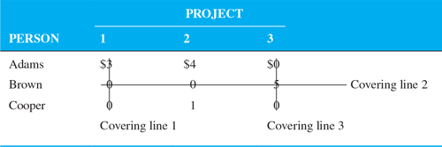
Table M8.20 illustrates that it is possible to cover all four zero entries in Table M8.19 with only two lines. Because there are three rows, an optimal assignment may not yet be made.
Table M8.20 Test for Optimal Solution to Fix-It Shop Problem

Step 3. Revise the Opportunity Cost Table.
An optimal solution is seldom obtained from the initial opportunity cost table. Often, we need to revise the table in order to shift one (or more) of the zero costs from its present location (covered by lines) to a new uncovered location in the table. Intuitively, we would want this uncovered location to emerge with a new zero opportunity cost.
This is accomplished by subtracting the smallest number not covered by a line from all numbers not covered by a straight line. This same smallest number is then added to every number (including zeros) lying at the intersection of any two lines.
The smallest uncovered number in Table M8.20 is 2, so this value is subtracted from each of the four uncovered numbers. A 2 is also added to the number that is covered by the intersecting horizontal and vertical lines. The results of step 3 are shown in Table M8.21.
Table M8.21 Revised Opportunity Cost Table for the Fix-It Shop Problem
| PROJECT | |||
|---|---|---|---|
| PERSON | 1 | 2 | 3 |
| Adams | $3 | $4 | $0 |
| Brown | 0 | 0 | 5 |
| Cooper | 0 | 1 | 0 |
To test now for an optimal assignment, we return to step 2 and find the minimum number of lines necessary to cover all zeros in the revised opportunity cost table. Because it requires three lines to cover the zeros (see Table M8.22), an optimal assignment can be made.
Table M8.22 Optimality Test on the Revised Fix-It Shop Opportunity Cost Table
Making the Final Assignment
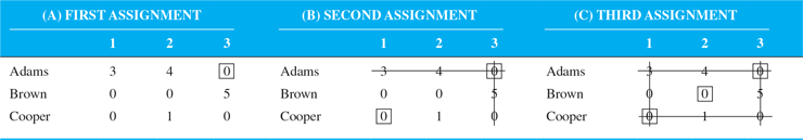
It is apparent that the Fix-It Shop problem’s optimal assignment is Adams to project 3, Brown to project 2, and Cooper to project 1. In solving larger problems, however, it is best to rely on a more systematic approach to making valid assignments. One such way is first to select a row or column that contains only one zero cell. Such a situation is found in the first row, Adams’s row, in which the only zero is in the project 3 column. An assignment can be made to that cell and then lines drawn through its row and column (see Table M8.23). From the uncovered rows and columns, we again choose a row or column in which there is only one zero cell. We make that assignment and continue the procedure until each person is assigned to one task.
Table M8.23 Making the Final Fix-It Shop Assignments
The total labor costs of this assignment are computed from the original cost table (see Table M8.17). They are as follows:
| ASSIGNMENT | COST ($) |
|---|---|
| Adams to project 3 | 6 |
| Brown to project 2 | 10 |
| Cooper to project 1 | 9 |
| Total cost | 25 |
Special Situations with the Assignment Algorithm
There are two special situations that require special procedures when using the Hungarian algorithm for assignment problems. The first involves solving problems that are not balanced, and the second involves solving a maximization problem instead of a minimization problem.
Unbalanced Assignment Problems
The solution procedure to assignment problems just discussed requires that the number of rows in the table equal the number of columns. Such a problem is called a balanced assignment problem. Often, however, the number of people or objects to be assigned does not equal the number of tasks or clients or machines listed in the columns, and the problem is unbalanced. When this occurs and we have more rows than columns, we simply add a dummy column or task (similar to how we handled unbalanced transportation problems earlier in this module). If the number of tasks that need to be done exceeds the number of people available, we add a dummy row. This creates a table of equal dimensions and allows us to solve the problem as before. Since the dummy task or person is really nonexistent, it is reasonable to enter zeros in its row or column as the cost or time estimate.
Suppose the owner of the Fix-It Shop realizes that a fourth worker, Davis, is also available to work on one of the three rush jobs that just came in. Davis can do the first project for $10, the second project for $13, and the third project for $8. The shop’s owner still faces the same basic problem—that is, which worker to assign to which project to minimize total labor costs. We do not have a fourth project, however, so we simply add a dummy column or dummy project. The initial cost table is shown in Table M8.24. One of the four workers, you should realize, will be assigned to the dummy project; in other words, the worker will not really be assigned any of the tasks.
Table M8.24 Estimated Project Repair Costs for Fix-It Shop with Davis Included
| PROJECT | ||||
|---|---|---|---|---|
| PERSON | 1 | 2 | 3 | DUMMY |
| Adams | $11 | $14 | $6 | $0 |
| Brown | 8 | 10 | 11 | 0 |
| Cooper | 9 | 12 | 7 | 0 |
| Davis | 10 | 13 | 8 | 0 |
Maximization Assignment Problems
Some assignment problems are phrased in terms of maximizing the payoff, profit, or effectiveness of an assignment instead of minimizing costs. It is easy to obtain an equivalent minimization problem by converting all numbers in the table to opportunity costs. This is brought about by subtracting every number in the original payoff table from the largest single number in that table. The transformed entries represent opportunity costs; it turns out that minimizing opportunity costs produces the same assignment as the original maximization problem. Once the optimal assignment for this transformed problem has been computed, the total payoff or profit is found by adding the original payoffs of those cells that are in the optimal assignment.
Let us consider the following example. The British navy wishes to assign four ships to patrol four sectors of the North Sea. In some areas, ships are to be on the lookout for illegal fishing boats, and in other sectors, they are to watch for enemy submarines, so the commander rates each ship in terms of its probable efficiency in each sector. These relative efficiencies are illustrated in Table M8.25. On the basis of the ratings shown, the commander wants to determine the patrol assignments producing the greatest overall efficiencies.
Table M8.25 Efficiencies of British Ships in Patrol Sectors
| SECTOR | ||||
|---|---|---|---|---|
| SHIP | A | B | C | D |
| 1 | 20 | 60 | 50 | 55 |
| 2 | 60 | 30 | 80 | 75 |
| 3 | 80 | 100 | 90 | 80 |
| 4 | 65 | 80 | 75 | 70 |
Step by step, the solution procedure is as follows. We first convert the maximizing efficiency table into a minimizing opportunity cost table. This is done by subtracting each rating from 100, the largest rating in the whole table. The resulting opportunity costs are given in Table M8.26.
Table M8.26 Opportunity Costs of British Ships
| SECTOR | |||||
|---|---|---|---|---|---|
| SHIP | A | B | C | D | |
| 1 | 80 | 40 | 50 | 45 | |
| 2 | 40 | 70 | 20 | 25 | |
| 3 | 20 | 0 | 10 | 20 | |
| 4 | 35 | 20 | 25 | 30 | |
We now follow steps 1 and 2 of the assignment algorithm. The smallest number in each row is subtracted from every number in that row (see Table M8.27); then the smallest number in each column is subtracted from every number in that column (as shown in Table M8.28).
Table M8.27 Row Opportunity Costs for the British Navy Problem
| SECTOR | |||||
|---|---|---|---|---|---|
| SHIP | A | B | C | D | |
| 1 | 40 | 0 | 10 | 5 | |
| 2 | 20 | 50 | 0 | 5 | |
| 3 | 20 | 0 | 10 | 20 | |
| 4 | 15 | 0 | 5 | 10 | |
Table M8.28 Total Opportunity Costs for the British Navy Problem
| SECTOR | |||||
|---|---|---|---|---|---|
| SHIP | A | B | C | D | |
| 1 | 25 | 0 | 10 | 0 | |
| 2 | 5 | 50 | 0 | 0 | |
| 3 | 5 | 0 | 10 | 15 | |
| 4 | 0 | 0 | 5 | 5 | |
The minimum number of straight lines needed to cover all zeros in this total opportunity cost table is four. Hence, an optimal assignment can be made already. You should be able by now to spot the best solution—namely, ship 1 to sector D, ship 2 to sector C, ship 3 to sector B, and ship 4 to sector A.
The overall efficiency, computed from the original efficiency data in Table M8.25, can now be shown:
| ASSIGNMENT | EFFICIENCY |
|---|---|
| Ship 1 to sector D | 55 |
| Ship 2 to sector C | 80 |
| Ship 3 to sector B | 100 |
| Ship 4 to sector A | 65 |
| Total efficiency | 300 |