CHAPTER 2

Neural Lazy Local Learning

J. M. VALLS, I. M. GALVÁN, and P. ISASI

Universidad Carlos III de Madrid, Spain

2.1 INTRODUCTION

Lazy learning methods [1–3] are conceptually straightforward approaches to approximating real- or discrete-valued target functions. These learning algorithms defer the decision of how to generalize beyond the training data until a new query is encountered. When the query instance is received, a set of similar related patterns is retrieved from the available training patterns set and is used to approximate the new instance. Similar patterns are chosen by means of a distance metric in such a way that nearby points have higher relevance.

Lazy methods generally work by selecting the k nearest input patterns from the query points. Usually, the metric used is the Euclidean distance. Afterward, a local approximation using the samples selected is carried out with the purpose of generalizing the new instance. The most basic form is the k-nearest neighbor method [4]. In this case, the approximation of the new sample is just the most common output value among the k examples selected. A refinement of this method, called weighted k-nearest neighbor [4], can also be used, which consists of weighting the contribution of each of the k neighbors according to the distance to the new query, giving greater weight to closer neighbors. Another strategy to determine the approximation of the new sample is locally weighted linear regression [2], which constructs a linear approximation of the target function over a region around the new query instance. The regression coefficients are based on the k nearest input patterns to the query.

By contrast, eager learning methods construct approximations using the entire training data set, and the generalization is carried out beyond the training data before observing the new instance. Artificial neural networks can be considered as eager learning methods because they construct a global approximation that covers the entire input space and all future query instances. That approximation over the training data representing the domain could lead to poor generalization properties, especially if the target function is complex or when data are not evenly distributed in the input space. In these cases, the use of a lazy strategy to train artificial neural networks could be appropriate because the complex target function could be described by a collection of less complex local approximations.

Bottou and Vapnik [5] have introduced a lazy approach in the context of artificial neural networks. The approach is based on the selection, for each query pattern, of the k closest examples from the training set. With these examples, a linear neural network classifier is trained to predict the test patterns. However, the idea of selecting the k nearest patterns might not be the most appropriate, mainly because the network will always be trained with the same number of training examples.

In this work we present a lazy learning approach for artificial neural networks. This lazy learning method recognizes from the entire training data set the patterns most similar to each new query to be predicted. The most similar patterns are determined by using weighting kernel functions, which assign high weights to training patterns close (in terms of Euclidean distance) to the new query instance received. The number of patterns retrieved will depend on the new query point location in the input space and on the kernel function, but not on the k parameter as in classical lazy techniques. In this case, selection is not homogeneous as happened in ref. 5; rather, for each testing pattern, it is determined how many training patterns would be needed and the importance in the learning process of each of them.

The lazy learning strategy proposed is developed for radial basis neural networks (RBNNs) [6,7]. It means that once the most similar or relevant patterns are selected, the approximation for each query sample is constructed by an RBNN. For this reason the method is called lazy RBNN (LRBNN). Other types of artificial neural networks could be used (e.g., the multilayer perceptron). However, RBNNs seem to be more appropriate for the low computational cost of training.

The chapter is organized as follows. Section 2.2 includes a detailed description of the lazy learning method proposed. In this section, two kernel weighting functions are presented: the Gaussian and inverse functions. Issues about the influence of using those kernel functions for making the selection of training patterns given a query instance are presented and analyzed. This section also includes the sequential procedure of the LRBNN method and two important aspects that must be taken into account when an RBNN is trained in a lazy way: random initialization of the RBNN parameters and the possibility of selecting no training patterns when the query point is located in certain regions of the input space. Section 2.3 covers the experimental validation of LRBNN. It includes a brief description of the domains used in the experiments as well as the results obtained using both kernel functions. Also in this section, LRBNN is compared with classical lazy techniques and with eager or classical RBNN. Finally, in Section 2.4 we draw conclusions regarding this work.

2.2 LAZY RADIAL BASIS NEURAL NETWORKS

The learning method presented consists of training RBNNs with a lazy learning approach [8,9]. As mentioned in Section 2.1, this lazy strategy could be applied to other types of artificial neural networks [10], but RBNNs have been chosen for the low computational cost of their training process. The method, called LRBNN (the lazy RBNN method), is based on the selection for each new query instance of an appropriate subset of training patterns from the entire training data set. For each new pattern received, a new subset of training examples is selected and an RBNN is trained to predict the query instance.

Patterns are selected using a weighting measure (also called a kernel function), which assigns a weight to each training example. The patterns selected are included one or more times in the resulting training subset and the network is trained with the most useful information, discarding those patterns that not only do not provide any knowledge to the network but that might confuse the learning process. Next, either the weighting measures for selecting the training patterns or the complete procedure to train an RBNN in a lazy way are explained. Also, some aspects related to the learning procedure are analyzed and treated.

2.2.1 Weighting Measures for Training Pattern Selection

Let us consider q, an arbitrary query instance, described by an n-dimensional vector and let X = {x_k, y_k}_{k=1, …,N} be the entire available training data set, where x_k is the input vector and y_k is the corresponding output. When a new instance q must be predicted, a subset of training patterns, named X_q, is selected from the entire training data set X.

In order to select X_q, which contains the patterns most similar to the query instance q, Euclidean distances (d_k) from all the training samples x_k to q must be evaluated. Distances may have very different magnitude depending on the problem domains, due to their different data values and number of attributes. It may happen that for some domains the maximum distance between patterns is many times the maximum distance between patterns for other domains. To make the method independent of the distance's magnitude, relative values must be used. Thus, a relative distance, d_rk, is calculated for each training pattern:

where d_max is the maximum distance to the query instance; this is d_max = max(d₁, d₂, …, d_N).

The selection of patterns is carried out by establishing a weight for each training pattern depending on its distance to the query instance q. That weight is calculated using a kernel function K(·), and it is used to indicate how many times a training pattern will be replicated into the subset X_q.

Kernel functions must reach their maximum value when the distance to the query point is null, and it decreases smoothly as this distance increases. Here we present and compare two kernel functions that fulfill the conditions above: the Gaussian and inverse functions, which are described next.

Weighted Selection of Patterns Using the Gaussian Function The Gaussian function assigns to each training pattern x_k a real value or weight according to

where σ is a parameter that indicates the width of the Gaussian function and d_rk is the relative Euclidean distance from the query to the training input pattern x_k given by Equation 2.1.

The weight values K(x_k), calculated in Equation 2.2, are used to indicate how many times the training pattern (x_k, y_k) will be included in the training subset associated with the new instance q. Hence, those real values must be transformed into natural numbers. The most intuitive way consists of taking the integer part of K(x_k). Thus, each training pattern will have an associated natural number given by

That value indicates how many times the pattern (x_k, y_k) is included in the subset X_q. If n_k = 0, the kth pattern is not selected and is not included in the set X_q.

Weighted Selection of Patterns Using the Inverse Function One problem that arises with the Gaussian function is its strong dependence on the parameter σ. For this reason, another weighting function, the inverse function, can be used:

This function does not depend on any parameter, but it is important to have some control over the number of training patterns selected. For this reason, an n-dimensional sphere centered at the test pattern is established in order to select only those patterns located in the sphere. Its radius, r, is a threshold distance, since all the training patterns whose distance to the novel sample is bigger than r will be discarded. To make it domain independent, the sphere radius will be relative with respect to the maximum distance to the test pattern. Thus, the relative radius, r_r, will be used to select the training patterns situated in the sphere centered at the test pattern, r_r being a parameter that must be established before employing the learning algorithm.

Due to the asymptotic nature of the inverse function, small distances could produce very large function values. For this reason, the values K(x_k) are normalized such that their sum equals the number of training patterns in X. These normalized values, denoted as K_n(x_k), are calculated in the following way:

where

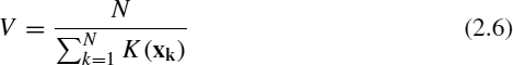
As in the case of the Gaussian function, the function values K_n(x_k) calculated in (2.5) are used to weight the selected patterns that will be used to train the RBNN. The main difference is that now, all the patterns located in the sphere, and only those, will be selected. Thus, both the relative distance d_rk calculated previously and the normalized weight value K_n(x_k) are used to decide whether the training pattern (x_k, y_k) is selected and, in that case, how many times it will be included in the training subset X_q. Hence, they are used to generate a natural number, n_k, following the next rule:

At this point, each training pattern in X has an associated natural number n_k (see Equation 2.7), which indicates how many times the pattern (x_k, y_k) will be used to train the RBNN for the new instance q. If the pattern is selected, n_k > 0; otherwise, n_k = 0.

Examples of these kernel functions (Gaussian and inverse) are presented in Figure 2.1. The x-axis represents the relative distance from each training example to the query, and the y-axis represents the value of the kernel function. When the Gaussian kernel function is used [see Figure 2.1(a)], the values of the function for patterns close to q are high and decrease quickly when patterns are moved away. Moreover, as the width parameter decreases, the Gaussian function becomes tighter and higher. Therefore, if the width parameter is small, only patterns situated very close to the new sample q are selected, and are repeated many times. However, when the width parameter is large, more training patterns are selected but they are replicated fewer times. We can observe that the value of σ affects the number of training patterns selected as well as the number of times they will be replicated.

If the selection is made using the inverse kernel function [see Figure 2.1(b)], the number of patterns selected depends only on the relative radius, r_r. Patterns close to the query instance q will be selected and repeated many times. As the distance to the query q increases, the number of times that training patterns are replicated decreases, as long as this distance is lower than r_r [in Figure 2.1(b), r_r has a value of 0.5]. If the distance is greater than r_r, they will not be selected. Figure 2.1(b) shows that the closest patterns will always be selected and replicated the same number of times, regardless of the radius value. This behavior does not happen with the Gaussian function, as we can see in Figure 2.1(a).

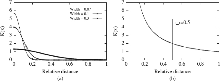
Figure 2.1 (a) Gaussian function with different widths; (b) inverse function and relative radius.

2.2.2 Training an RBNN in a Lazy Way

Here, we present the LRBNN procedure. For each query instance q:

1. The standard Euclidean distances d_k from the pattern q to each input training pattern are calculated.
2. The relative distances d_rk, given by Equation 2.1, are calculated for each training pattern.
3. A weighting or kernel function is chosen and the n_k value for each training pattern is calculated. When the Gaussian function is used, the n_k values are given by Equation 2.3, and for the inverse function they are calculated using Equation 2.7.
4. The training subset X_q is obtained according to value n_k for each training pattern. Given a pattern (x_k, y_k) from the original training set X, that pattern is included in the new subset if the value n_k is higher than zero. In addition, the pattern (x_k, y_k) is placed in the training set X_q n_k times in random order.
5. The RBNN is trained using the new subset X_q. The training process of the RBNN implies the determination of the centers and dilations of the hidden neurons and the determination of the weights associated with those hidden neurons to the output neuron. Those parameters are calculated as follows:

   (a) The centers of neurons are calculated in an unsupervised way using the K-means algorithm in order to cluster the input space formed by all the training patterns included in the subset X_q, which contains the replicated patterns selected.

   (b) The neurons dilations or widths are evaluated as the geometric mean of the distances from each neuron center to its two nearest centers.

   (c) The weights associated with the connections from the hidden neurons to the output neuron are obtained, in an iterative way, using the gradient descent method to minimize the mean-square error measured in the output of the RBNN over the training subset X_q.

2.2.3 Some Important Aspects of the LRBNN Method

To apply the lazy learning approach, two features must be taken into account. On the one hand, the results would depend on the random initialization of the K-means algorithm, which is used to determine the locations of the RBNN centers. Therefore, running the K-means algorithm with different random initialization for each test sample would have a high computational cost.

On the other hand, a problem arises when the test pattern belongs to regions of the input space with a low data density: It could happen that no training example would be selected. In this case, the method should offer some alternative in order to provide an answer for the test sample. We present solutions to both problems.

K-Means Initialization Given the objective of achieving the best performance, a deterministic initialization is proposed instead of the usual random initializations. The idea is to obtain a prediction of the network with a deterministic initialization of the centers whose accuracy is similar to the one obtained when several random initializations are done. The initial location of the centers will depend on the location of the closest training examples selected. The deterministic initialization is obtained as follows:

• Let (x₁, x₂, …, x₁) be the l training patterns selected, ordered by their values (K(x₁), K(x₂), …, K(x₁)) when the Gaussian function is used (Equation 2.2) or their normalized values when the selection is made using the inverse function calculated in Equation 2.5:

  (K_n(x₁), K_n(x₂), …, K_n(x_l))

• Let m be the number of hidden neurons of the RBNN to be trained.
• The center of the ith neuron is initialized to the x_i position for i = 1, 2, …, m.

It is necessary to avoid situations where m > l. The number of hidden neurons must be fixed to a number smaller than the patterns selected, since the opposite would not make any sense.

Empty Training Set It has been observed that when the input space data are highly dimensional, in certain regions of it the data density can be so small that any pattern is selected. When this situation occurs, an alternative method to select the training patterns must be used. Here we present two different approaches.

1. If the subset X_q associated with a test sample q is empty, we apply the method of selection to the closest training pattern as if it were the test pattern. In more detail: Let x_c be the closest training pattern to q. Thus, we will consider x_c the new test pattern, being named q′. We apply our lazy method to this pattern, generating the X_q′ training subset. Since q′ ∈ X, X_q′ will always have at least one element. At this point the network is trained with the set X_q′ to answer to the test point q.
2. If the subset X_q associated with a test sample q is empty, the network is trained with X, the set formed by all the training patterns. In other words, the network is trained as usual, with all the patterns available.

As mentioned previously, if no training examples are selected, the method must provide some answer to the test pattern. Perhaps the most intuitive solution consists of using the entire training data set X; this alternative does not have disadvantages since the networks will be trained, in a fully global way, with the entire training set for only a few test samples. However, to maintain the coherence of the idea of training the networks with some selection of patterns, we suggest the first alternative. The experiments carried out show that this alternative behaves better.

2.3 EXPERIMENTAL ANALYSIS

The lazy strategy described above, with either the Gaussian or the inverse kernel function, has been applied to different RBNN architectures to measure the generalization capability of the networks in terms of the mean absolute error over the test data. We have used three domains to compare the results obtained by both kernel functions when tackling different types of problems. Besides, we have applied both eager RBNN and classical lazy methods to compare our lazy RBNN techniques with the classical techniques. The classical lazy methods we have used are k-nearest neighbor, weighted k-nearest neighbor, and weighted local regression.

2.3.1 Domain Descriptions

Three domains have been used to compare the different lazy strategies. Two of them are synthetic problems and the other is a real-world time series domain. The first problem consists of approximating the Hermite polynomial. This is a well-known problem widely used in the RBNN literature [11,12]. A uniform random sampling over the interval [−4, 4] is used to obtain 40 input–output points for the training data. The test set consists of 200 input–output points generated in the same way as the points in the training set.

The next domain corresponds to the Mackey–Glass time series prediction and is, as the former one, widely regarded as a benchmark for comparing the generalization ability of an RBNN [6,12]. It is a chaotic time series created by the Mackey–Glass delay-difference equation [13]:

The series has been generated using the following values for the parameters: a = 0.2, b = 0.1, and τ = 17. The task for the RBNN is to predict the value x[t + 1] from the earlier points (x[t], x[t − 6], x[t − 12], x[t − 18]). Fixing x(0) = 0, 5000 values of the time series are generated using Equation (2.8). To avoid the initialization transients, the initial 3500 samples are discarded. The following 1000 data points have been chosen for the training set. The test set consists of the points corresponding to the time interval [4500, 5000].

Finally, the last problem, a real-world time series, consists of predicting the water level at Venice lagoon [14]. Sometimes, in Venice, unusually high tides are experienced. These unusual situations are called high water. They result from a combination of chaotic climatic elements in conjunction with the more normal, periodic tidal systems associated with that particular area. In this work, a training data set of 3000 points, corresponding to the level of water measured each hour, has been extracted from available data in such a way that both stable situations and high-water situations appear represented in the set. The test set has also been extracted from the data available and is formed of 50 samples, including the high-water phenomenon. A nonlinear model using the six previous sampling times seems appropriate because the goal is to predict only the next sampling time.

2.3.2 Experimental Results: Lazy Training of RBNNs

When RBNNs are trained using a lazy strategy based on either the Gaussian or the inverse kernel function to select the most appropriate training patterns, some conditions must be defined. Regarding the Gaussian kernel function, experiments varying the value of the width parameter from 0.05 to 0.3 have been carried out for all the domains. That parameter determines the shape of the Gaussian and therefore, the number of patterns selected to train the RBNN for each testing pattern. Those maximum and minimum values have been chosen such that the shape of the Gaussian allows selection of the same training patterns, although in some cases no training patterns might be selected. For the inverse selective learning method, and for reasons similar to those for the Gaussian, different values of the relative radius have been set, varying from 0.04 to 0.24 for all the domains. In addition, experiments varying the number of hidden neurons have been carried out to study the influence of that parameter in the performance of the method.

As noted in Section 2.2.3, two issues must be considered when employing the lazy learning approach. First, the results would depend on the random initialization of the RBNN centers used by the K-means algorithm. Thus, running the K-means algorithm with different random initializations for each testing pattern would be computationally expensive. To avoid this problem, we propose a deterministic initialization of the K-means algorithm. Second, when the testing pattern belongs to input space regions with a low data density, it might happen that no training example was selected. In this case, as we explained earlier, the method offers two alternatives for providing an answer to the query sample.

To evaluate the deterministic initialization proposed and compare it with the usual random initialization we have developed experiments for all the domains using the lazy learning approach when the neurons centers are randomly initialized. Ten runs have been made and we have calculated the mean values of the corresponding errors. We have also applied the proposed deterministic initialization.

The results show that for all the domains studied, the errors are similar or slightly better. That is, when we carry out the deterministic initialization, the errors are similar to the mean of the errors obtained when 10 different random initializations are made. For instance, in Table 2.1 we show the mean of these errors (10 random initializations) for the Mackey–Glass time series when the inverse selection function is used for different RBNN architectures and relative radius (the standard deviations for these 10 error values are shown in Table 2.2). Table 2.3 shows the results obtained for the Mackey–Glass time series when the deterministic initialization is used. Values lower than the corresponding errors in Table 2.1 are shown in boldface. We can observe that the error values are slightly better than those obtained when the neuron centers were located randomly. Thus, we can use the deterministic initialization instead of several random initializations, reducing the computational cost.

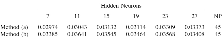
In Tables 2.1 and 2.3 the column NP displays the number of null patterns, that is, test patterns for which the number of training patterns selected is zero. As explained in Section 2.2.3, two alternative ways of treating these anomalous patterns are presented. Method (a) retains the local approach, and method (b) renounces the local approach and follows a global one, assuming that the entire training set must be taken into account.

TABLE 2.1 Mean Errors with Random Initialization of Centers: Mackey–Glass Time Series

TABLE 2.2 Standard Deviations of Errors Corresponding to 10 Random Initializations of Centers: Mackey–Glass Time Series

TABLE 2.3 Errors with Deterministic Initialization of Centers: Mackey–Glass Time Series

When null patterns are found, we have tested both approaches. After experiments in all domains, we have concluded that it is preferable to use method (a) [9], not only because it behaves better but also because it is more consistent with the idea of training the networks with a selection of patterns. For instance, for the Mackey–Glass domain with the inverse kernel function, 45 null patterns are found when r_r = 0.04 (see Table 2.3). Table 2.4 shows error values obtained for both methods, and we observe that errors are better when method (a) is used.

TABLE 2.4 Errors with Deterministic Initialization of Centers and Null Pattern Processing (r_r = 0.04): Mackey–Glass Time Series

Next, we summarize the results obtained for all the domains, for both the inverse and the Gaussian selection functions, using the deterministic initialization in all cases and method (a) if null patterns are found. Figures 2.2, 2.3 and 2.4 show for the three application domains the behavior of the lazy strategy when the Gaussian and inverse kernel function are used to select the training patterns. In those cases, the mean error over the test data is evaluated for every value of the width for the Gaussian case and for every value of the relative radius for the inverse case. These figures show that the performance of the lazy learning method proposed to train RBNNs does not depend significantly on the parameters that determine the number of patterns selected when the selection is based on the inverse kernel function. With the inverse function and for all application domains, the general tendency is that there exists a wide interval of relative radius values, r_r, in which the errors are very similar for all architectures. Only when the r_r parameter is fixed to small values is generalization of the method poor in some domains. This is due to the small number of patterns selected, which is not sufficient to construct an approximation. However, as the relative radius increases, the mean error decreases and then does not change significantly. Additionally, it is observed that the number of hidden neurons is not a critical parameter in the method.

Figure 2.2 Errors with (a) Gaussian and (b) inverse selection for the Hermite polynomial.

Figure 2.3 Errors with (a) Gaussian and (b) inverse selection for the Mackey–Glass time series.

Figure 2.4 Errors with (a) Gaussian and (b) inverse selection for lagoon-level prediction.

When Gaussian selection is used, the performance of the method presents some differences. First, although there is also an interval of width values in which the errors are similar, if the width is fixed to high values, the error increases. For those values, the Gaussian is flatter and it could also happen that an insufficient number of patterns are selected. Second, in this case, the architecture of the RBNN is a more critical factor in the behavior of the method.

2.3.3 Comparative Analysis with Other Classical Techniques

To compare the proposed method with classical techniques related to our approach, we have performed two sets of experiments over the domains studied, in one case using eager RBNN and in the other, well-known lazy methods. In the first set we have used different RBNN architectures trained with all the available training patterns to make the predictions on the test sets; in the second set of experiments, we have applied to the domains studied the following classical lazy methods: k-nearest neighbor, weighted k-nearest neighbor, and weighted local regression. In all cases, we have measured the mean absolute error over the test data sets.

Regarding classical RBNN, different architectures, from 10 to 130 neurons, have been trained for all the domains in an eager way, using the entire training data set. The best mean errors over the test set for all the domains obtained by the various methods (lazy RBNN, eager RBNN) are shown in Table 2.5. The table shows that the generalization capability of RBNNs increases when they are trained using a lazy strategy instead of the eager or traditional training generally used in the context of neural networks. The results improve significantly when the selection is based on the input information contained in the test pattern and when this selection is carried out with the inverse function.

With respect to the second set of experiments using the classical lazy methods, k-nearest neighbor, weighted k-nearest neighbor, and weighted local regression methods [2] have been run for different values of the k parameter (number of patterns selected). Table 2.6 shows the best mean errors (and the corresponding k-parameter value) obtained by these methods for all the domains.

TABLE 2.5 Best Error for the Lazy Strategy to Train RBNNs Compared with Traditional Training

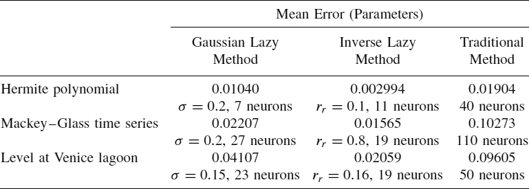
TABLE 2.6 Best Error for k-Nearest Neighbor, Weighted k-Nearest Neighbor, and Linear Local Regression Methods

Tables 2.5 and 2.6 show that the lazy training of RBNNs using the inverse selection function improves the performance of traditional lazy methods significantly. This does not happen when the Gaussian selection function is used: The errors are better than those obtained by traditional lazy methods, but not in all cases. Therefore, the selection function becomes a key issue in the performance of the method.

2.4 CONCLUSIONS

Machine learning methods usually try to learn some implicit function from the set of examples provided by the domain. There are two ways of approaching this problem. On the one hand, eager or global methods build up an approximation using all available training examples. Afterward, this approximation will allow us to forecast any testing query. Artificial neural networks can be considered as eager learning methods because they construct a global approximation that covers the entire input space and all future query instances. However, in many domains with nonhomogeneous behavior where the examples are not evenly distributed in the input space, these global approximations could lead to poor generalization properties.

Lazy methods, on the contrary, build up a local approximation for each testing instance. These local approximations would adapt more easily to the specific characteristics of each input space region. Therefore, for those types of domains, lazy methods would be more appropriate. Usually, lazy methods work by selecting the k nearest input patterns (in terms of Euclidean distance) from the query points. Afterward, they build the local approximation using the samples selected in order to generalize the new query point. Lazy methods show good results, especially in domains with mostly linear behavior in the regions. When regions show more complex behavior, those techniques produce worse results.

We try to complement the good characteristics of each approach by using lazy learning for selecting the training set, but using artificial neural networks, which show good behavior for nonlinear predictions, to build the local approximation. Although any type of neural model can be used, we have chosen RBNNs, due to their good behavior in terms of computational cost.

In this work we present two ways of doing pattern selection by means of a kernel function: using the Gaussian and inverse functions. We have compared our approach with various lazy methods, such as k-nearest neighbor, weighted k-nearest neighbor, and local linear regression. We have also compared our results with eager or classical training using RBNNs.

One conclusion of this work is that the kernel function used for selecting training patterns is relevant for the success of the network since the two functions produce different results. The pattern selection is a crucial step in the success of the method: It is important to decide not only what patterns are going to be used in the training phase, but also how those patterns are going to be used and the importance of each pattern in the learning phase. In this work we see that the Gaussian function does not always produce good results. In the validation domains, the results are rather poor when the selection is made using the Gaussian function, although they are better than the results obtained using traditional methods. However, they are always worse than when the inverse function is used. This function has good results in all domains, also improving the results obtained using classical lazy techniques. Besides, the proposed deterministic initialization of the neuron centers produces results similar to those from the usual random initialization, thus being preferable because only one run is necessary. Moreover, the method is able to predict 100% of the test patterns, even in those extreme cases when no training examples are selected.

Summarizing, the results show that the combination of lazy learning and RBNN improves eager RBNN learning substantially and could reach better results than those of other lazy techniques. Two different aspects must be taken into consideration: first, we need a good method (compatible with lazy approaches) for selecting training patterns for each new query; and second, a nonlinear method must be used for prediction. The regions may have any type of structure, so a general method will be required.

Acknowledgments

This work has been financed by the Spanish-funded MCyT research project OPLINK, under contract TIN2005-08818-C04-02.

REFERENCES

1. D. W. Aha, D. Kibler, and M. Albert. Instance-based learning algorithms. Machine Learning, 6:37–66, 1991.

2. C. G. Atkeson, A. W. Moore, and S. Schaal. Locally weighted learning. Artificial Intelligence Review, 11:11–73, 1997.

3. D. Wettschereck, D. W. Aha, and T. Mohri. A review and empirical evaluation of feature weighting methods for a class of lazy learning algorithms. Artificial Intelligence Review, 11:273–314, 1997.

4. B.V. Dasarathy, ed. Nearest Neighbor (NN) Norms: NN Pattern Classification Techniques. IEEE Computer Society Press, Los Alamitos, CA, 1991.

5. L. Bottou and V. Vapnik. Local learning algorithms. Neural Computation, 4(6):888–900, 1992.

6. J. E. Moody and C. J. Darken. Fast learning in networks of locally-tuned processing units. Neural Computation, 1:281–294, 1989.

7. T. Poggio and F. Girosi. Networks for approximation and learning. Proceedings of the IEEE, 78:1481–1497, 1990.

8. J. M. Valls, I. M. Galván, and P. Isasi. Lazy learning in radial basis neural networks: a way of achieving more accurate models. Neural Processing Letters, 20(2):105–124, 2004.

9. J. M. Valls, I. M. Galván, and P. Isasi. LRBNN: a lazy RBNN model. AI Communications, 20(2):71–86, 2007.

10. I. M. Galván, P. Isasi, R. Aler, and J. M. Valls. A selective learning method to improve the generalization of multilayer feedforward neural networks. International Journal of Neural Systems, 11:167–157, 2001.

11. A. Leonardis and H. Bischof. An efficient MDL-based construction of RBF networks. Neural Networks, 11:963–973, 1998.

12. L. Yingwei, N. Sundararajan, and P. Saratchandran. A sequential learning scheme for function approximation using minimal radial basis function neural networks. Neural Computation, 9:461–478, 1997.

13. M. C. Mackey and L. Glass. Oscillation and chaos in physiological control systems. Science, 197:287–289, 1997.

14. J. M. Zaldívar, E. Gutiérrez, I. M. Galván, F. Strozzi, and A. Tomasin. Forecasting high waters at Venice lagoon using chaotic time series analysis and nonlinear neural networks. Journal of Hydroinformatics, 2:61–84, 2000.