CHAPTER 6

Canonical Metaheuristics for Dynamic Optimization Problems

G. LEGUIZAMÓN, G. ORDÓÑEZ, and S. MOLINA

Universidad Nacional de San Luis, Argentina

E. ALBA

Universidad de Málaga, Spain

6.1 INTRODUCTION

Many real-world optimization problems have a nonstationary environment; that is, some of their components depend on time. These types of problems are called dynamic optimization problems (DOPs). Dynamism in real-world problems can be attributed to several factors: some are natural (e.g., weather conditions); others can be related to human behavior (e.g., variation in aptitude of different individuals, inefficiency, absence, and sickness); and others are business related (e.g., the addition of new orders and cancellation of old ones). Techniques that work for static problems may therefore not be effective for DOPs, which require algorithms that make use of old information to find new optima quickly. An important class of techniques for static problems are the metaheuristics (MHs), the most recent developments in approximate search methods for solving complex optimization problems [21].

In general, MHs guide a subordinate heuristic and provide general frameworks that allow us to create new hybrids by combining different concepts derived from classical heuristics, artificial intelligence, biological evolution, natural systems, and statistical mechanical techniques used to improve their performance. These families of approaches include, but are not limited to, evolutionary algorithms, particle swarm optimization, ant colony optimization, differential evolution, simulated annealing, tabu search, and greedy randomized adaptive search process. It is remarkable that MHs have been applied successfully to stationary optimization problems. However, there also exists increasing research activity on new developments of MHs applied to DOPs with encouraging results.

In this chapter we focus on describing the use of population-based MHs (henceforth, called simply MHs) from a unifying point of view. To do that, we first give a brief description and generic categorization of DOPs. The main section of the chapter is devoted to the application of canonical MHs to DOPs, including general suggestions concerning the way in which they can be implemented according to the characteristic of a particular DOP. This section includes an important number of references of specific proposals about MHs for DOPs. The two last sections are devoted, respectively, to considerations about benchmarks and to typical metrics used to assess the performance of MHs for DOPs. Finally, we draw some conclusions.

6.2 DYNAMIC OPTIMIZATION PROBLEMS

DOPs are optimization problems in which some of the components depend on time; that is, there exists at least one source of dynamism that affects the objective function (its domain, its landscape, or both). However, the mere existence of a time dimension in a problem does not mean that the problem is dynamic. Problems that can be solved ahead of time are not dynamic even though they might be time dependent. According to Abdunnaser [1], Bianchi [4], Branke [11], and Psaraftis [36], the following features can be found in most real-world dynamic problems: (1) the problem can change with time in such a way that future scenarios are not known completely, yet the problem is known completely up to the current moment without any ambiguity about past information; (2) a solution that is optimal or nearly optimal at a certain time may lose its quality in the future or may even become infeasible; (3) the goal of the optimization algorithm is to track the shifting optima through time as closely as possible; (4) solutions cannot be determined ahead of time but should be found in response to the incoming information; and (5) solving the problem entails setting up a strategy that specifies how the algorithm should react to environmental changes (e.g., to solve the problem from scratch or adapt some parameters of the algorithm at every change).

The goal in stationary optimization problems is to find a solution s* that maximises the objective function O (note that maximizing a function O is the same as minimizing −O):

where S is the set of feasible solutions and is the objective function. On the other hand, for DOPs the set of feasible solutions and/or the objective function depends on time; therefore, the goal at time t is to find a solution s* that fulfills

where at time t₁, set S(t) is defined for all t ≤ t₁ and O(s, t) is fully defined for s ∈ S(t) ∧ t ≤ t₁; however, there exists uncertainty for S(t) and/or O(s, t) values for t > t₁. This uncertainty is required to consider a problem as dynamic. Nevertheless, instances of dynamic problems used in many articles to test algorithms are specified without this type of uncertainty, and changes are generated following a specific approach (see Section 6.3). Additionally, the particular algorithm used to solve DOPs is not aware of these changes and the way they are generated. Consequently, from the point of view of the algorithm, these are real DOP instances satisfying the definition above.

Regarding the above, the specification of a DOP instance should include (1) an initial state [conformed of the definition of S(0) and a definition of O(s, 0) for all s ∈ S(t)], (2) a list of sources of dynamism, and (3) the specifications of how each source of dynamism will affect the objective function and the set of feasible solutions. Depending on the sources of dynamism and their effects on the objective function, DOPs can be categorized in several ways by answering such questions as “what” (aspect of change), “when” (frequency of change), and “how” (severity of change, effect of the algorithm over the scenario, and presence of patterns). Each of these characteristics of DOPs is detailed in the following subsections.

6.2.1 Frequency of Change

The frequency of change denotes how often a scenario is modified (i.e., is the variation in the scenario continuous or discrete?). For example, when discrete changes occur, it is important to consider the mean time between consecutive changes. According to these criteria and taking into account their frequency, two broad classes of DOPs can be defined as follows:

1. Discrete DOPs. All sources of dynamism are discrete; consequently, for windowed periods of time, the instance seems to be a stationary problem. When at some time new events occur, they make the instance behave as another stationary instance of the same problem. In other words, DOPs where the frequency of change is discrete can be seen as successive and different instances of a stationary problem, called stages.

Example 6.1 (Discrete DOP) Let us assume an instance of a version of the dynamic traveling salesman problem (DTSP) where initially the salesman has to visit n cities; however, 10 minutes later, he is informed that he has to visit one more city; in this case the problem behaves as a stationary TSP with n cities for the first 10 minutes, and after that it behaves as a different instance of the stationary TSP, with n + 1 cities.

2. Continuous DOPs. At least one source of dynamism is continuous (e.g., temperature, altitude, speed).

Example 6.2 (Continuous DOP) In the moving peaks problem [9,10] the objective function is defined as

where s is a vector of real numbers that represents the solution, B(s) a time-invariant basis landscape, P a function defining the peak shape, m the number of peaks, and each peak has its own time-varying parameter: height (h_i), width (w_i), and location (p_i). In this way each time we reevaluate solution s the fitness could be different.

6.2.2 Severity of Change

The severity of change denotes how strong changes in the system are (i.e., is it just a slight change or a completely new situation?) In discrete DOPs, severity refers to the differences between two consecutive stages.

Example 6.3 (Two Types of Changes in DTSP) Let us suppose a DTSP problem with 1000 cities, but that after some time a new city should be incorporated in the tour. In this case, with a high probability, the good-quality solutions of the two stages will be similar; however, if after some time, 950 out of 1000 cities are replaced, this will generate a completely different scenario.

6.2.3 Aspect of Change

The aspect of change indicates what components of the scenario change: the optimization function or some constraint. There exist many categorizations of a DOP, depending on the aspect of change. Basically, a change could be in one of the following categories:

• Variations in the values of the objective function (i.e., only the objective values are affected). Thus, the goal is to find a solution s* that fulfills the equation

  

• Variations in the set of feasible solutions (i.e., only the set of problem constraints are affected). Thus, the goal is to find a solution s* that fulfills the equation

  

  In this case, a possible change in S(t) will make feasible solutions infeasible, and vice versa.

• Variations in both of the components above, which is the most general case, and the goal is to find a solution s* that fulfills Equation 6.2.

6.2.4 Interaction of the Algorithm with the Environment

Up to this point we have assumed that all the sources of dynamism are external, but for some problems the algorithm used to approach them is able to influence the scenario. In this way, DOPs can be classified [6] as (a) control influence: the algorithms used to tackle the problem have no control over the scenario (i.e., all sources of dynamism are external); and (b) system influence: the algorithms used to tackle the problem have some control over the scenario (i.e., the algorithms themselves incorporate an additional source of dynamism).

Example 6.4 (System Influence DOP) Let us assume that we have a production line with several machines, where new tasks arrive constantly to be processed by some of the machines. The algorithm chosen produces a valid schedule, but after some time a machine idle event is generated. The best solution known so far is used to select and assign the task to the idle machine. In this way the task assigned (selected by the algorithm) is no longer on the list of tasks to be scheduled (i.e., the algorithm has changed the scenario).

6.2.5 Presence of Patterns

Even if the sources of dynamism are external, the sources sometimes show patterns. Therefore, if the algorithm used to tackle the DOP is capable of detecting this situation, it can take some advantage to react properly to the new scenario [7,8,39]. Some characteristics of MHs make them capable of discovering some patterns about situations associated with the possible changes in the scenario and, additionally, keeping a set of solutions suitable for the next stage. In this way, when a change occurs, the MH could adapt faster to the newer situation. However, sometimes it is not possible to predict a change but it is still possible to predict when it will be generated. In these cases, a possible mechanism to handle the changes is to incorporate in the fitness function a measure of solution flexibility (see Section 6.3) to reduce the adapting cost to the new scenario [13]. Furthermore, a common pattern present in many DOPs, especially in theoretical problems, is the presence of cycles (an instance has cycles if the optimum returns to previous locations or achieves locations close to optimum).

Example 6.5 (Presence of Cycles) A classic DOP that fits in this category is a version of the dynamic knapsack problem [22], where the problem switches indefinitely between two stages.

6.3 CANONICAL MHs FOR DOPs

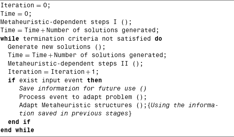
Algorithm 6.1 shows the skeleton of the most traditional population-based MHs for solving stationary problems as defined in Equation 6.2. However, its application to DOPs needs incorporation of the concept of time either by using an advanced library to handle real-time units or by using the number of evaluations [11], which is the more widely used method. When considering the number of evaluations, Algorithm 6.1 should be adapted to include dynamism in some way, as shown in Algorithm 6.2, which represents a general outline of an MH to handle the concept of time. However, the objective is not the same for stationary problems as for DOPs. Whereas in stationary problems the objective is to find a high-quality solution, in DOPs there exists an additional objective, which is to minimize the cost of adapting to the new scenario; that is, there are two opposing objectives: solution quality and adaptation cost. The first is similar to the fitness functions used with stationary problems and represents the quality of the solution at a specific time; the second is focused on evaluating the adaptation capacity of the algorithm when the scenario has changed.

Algorithm 6.1 Static MH

Algorithm 6.2 DMH: Time Concept Incorporation

The first step is to determine the way in which the MHs will react when facing a new scenario. If considering discrete DOPs, the stages can be seen as independent stationary problems (see Section 6.2.1). In this case, a reinitialization step takes place when a particular event changes the scenario (see Algorithm 6.3). When these two stages are similar, it makes no sense to discard all the information obtained so far; therefore, an alternative to the reinitialization process is to reuse the information collected and adapt it to the new stage (see Algorithm 6.4). These two algorithms have been widely used in different studies and it has been shown that Algorithm 6.4 performs significantly better than Algorithm 6.3 in most situations; however, some authors suggest that for problems with a high frequency of change, Algorithm 6.3 outperforms ref. 11. As a general rule, it can be said that for both low values of frequency and severity of change, Algorithm 6.4 outperforms Algorithm 6.3.

Algorithm 6.3 DMH: Reinitialization

Algorithm 6.4 DMH: Reuse Information

On the other hand, in continuous DOPs, each time a solution is evaluated the scenario could be different. Therefore, Algorithm 6.3 is not suitable for these types of problems, and similarly, Algorithm 6.4 cannot be applied directly. To do that, it is necessary to consider the aspect of change and the particular MH. To adapt Algorithm 6.4 for continuous DOPs, lines 10 to 13 should be moved into either “Generate new solutions” or “Metaheuristic-dependent steps II,” according to the MH. A common approach when the severity of change is low is to ignore these changes for discrete periods of time and proceed as if solving a discrete DOP.

Although the second strategy (represented by Algorithm 6.4) is more advanced than the first (represented by Algorithm 6.3), the second has better convergence properties, which, indeed, are useful in stationary problems, but when solving DOPs, those properties can be a serious drawback, due to the lack of diversity. There are two principal approaches to augmenting population diversity: reactive and proactive [43]. The reactive approach consists of reacting to a change by triggering a mechanism to increase the diversity, whereas the proactive approach consists of maintaining population diversity through the entire run of the algorithm. In the following, some examples of these two approaches are listed.

• Reactive approaches: hypermutation [15], variable local search [40], shaking [18], dynamic updating of the MH parameters to intensify either exploration or exploitation [42,43], turbulent particle swarm optimization [26], pheromone conservation procedure [17].
• Proactive approaches: random immigrants [23], sharing/crowding [2,14], thermodynamical GA [31], sentinels [33], diversity as second objective [29], speciation-based PSO (SPSO) [27,28].
• Reactive and/or proactive approaches (multipopulation): maintain different subpopulations on different regions [11], self-organizing scouts [11,12] multinational EA [38], EDA multipopulation approach with random migration [30], multiswarm optimization in dynamic environments [5].

It is worth remarking that for the different MHs there exist different alternatives for implementing approaches to handling diversity. However, particular implementations should avoid affecting the solution quality (e.g., an excessive diversity will avoid a minimum level of convergence, also needed when facing DOPs).

Another important concept in MHs for DOPs is solution flexibility. A solution can be considered flexible if after a change in the scenario, its fitness is similar to that of the preceding stage. Clearly, flexibility is an important and desirable feature for the solutions which allow the MHs to lower the adaptation cost. To generate solutions as flexible as possible, the following approaches can be considered:

• Multiobjective. The MH is designed to optimize two objectives, one represented by the original fitness function and the other by a metric value indicating solution flexibility [12].
• Dynamic fitness. When the time to the next change is known or can be estimated, the fitness function is redefined as

  

  where F(x) is the old fitness function, Flex(x) measures the solution flexibility, and a(t) ∈ [0, 1] is an increasing function except when changes occur. In this way, function a is designed such that (a) when the time for the next change is far away, it gives very low values (i.e., solutions with higher fitness values are preferred); and (b) when approaching the next change, it gives higher values in order to prefer more flexible solutions.

In addition, the literature provides plenty of specific techniques for specific classes of DOPs approached by means of MHs. For instance, for DOPs that show similar or identical cyclical stages, it could be useful to consider an approach that uses implicit or explicit memory to collect valuable information to use in future stages (Algorithm 6.5 shows the overall idea of an MH that uses explicit memory). On the other hand, algorithms proposed for system control DOPs have been developed [6]. Other authors have redefined a MH specifically designed to be used for DOPs (e.g, the population-based ACO) [24,25].

Algorithm 6.5 DMH: With Explicit Memory

6.4 BENCHMARKS

Benchmarks are useful in comparing optimization algorithms to highlight their strengths, expose their weaknesses, and to help in understanding how an algorithm behaves [1]. Therefore, selection of an adequate benchmark should take into account at least how to (1) specify and generate a single instance and (2) select an appropriate set of instances.

6.4.1 Instance Specification and Generation

As mentioned earlier, DOP instances are defined as (a) an initial state, (b) a list of sources of dynamism, and (c) the specification of how each source of dynamism will affect the objective function and/or the set of feasible solutions. However, for a particular benchmark the behavior of the sources of dynamism has to be simulated. To do that, two approaches can be considered: use of (1) a stochastic event generator or (2) a predetermined list of events. The instances modeled using a stochastic event generator generally have the advantage that they are parametric and allow us to have a wide range of controlled situations. On the other hand, instances that use a predetermined list of events allow us to repeat the experiments, which provides some advantages for the statistical test. If all the sources of dynamism are external (control influence DOPs), it is a good idea to use the stochastic event generator to create a list of events. In addition, it is worth remarking that the researcher could know beforehand about the behavior of the instances for all times t; in real-life situations, only past behavior is known. Therefore, algorithms used to tackle the problem should not take advantage of knowledge of future events.

6.4.2 Selection of an Adequate Set of Benchmarks

When defining a new benchmark we must take into account the objective of our study: (a) to determine how the dynamic problem components affect the performance of a particular MH, or (b) to determine the performance of a particular MH for a specific problem. Although these are problem-specific considerations, it is possible to give some hints as to how to create them.

For the first case it is useful to have a stochastic instance generator that allows us to specify as many characteristics of the instances as possible (i.e., frequency of change, severity of change, etc.). However, to analyze the impact of a specific characteristic on an MH, it is generally useful to choose one characteristic and fix the remaining ones. In this situation, a possible synergy among the characteristics must be taken into account (i.e., sometimes the effect of two or more characteristics cannot be analyzed independently). On the other hand, when comparing the performance of an MH against other algorithms or MHs, it is useful to consider existing benchmarks when available. As an example, Table 6.1 displays a set of well-known benchmarks for different DOPs. Only when no benchmark is available or when an available benchmark is not adequate for the problem considered is it necessary to generate a new benchmark considering at least the inclusion of instances: (a) with different characteristics to cover the maximum number of situations with a small set of instances (the concept of synergy is also very important here), (b) with extreme and common characteristics, and (c) that avoids being tied to a specific algorithm.

TABLE 6.1 Examples of Benchmarks

Problem	Reference
Dynamic bit matching	[35]
Moving parabola	[3]
Time-varying knapsack	[22]
Moving peaks	[34]
Dynamic job shop scheduling	[19]

6.5 METRICS

To analyze the behavior of an MH applied to a specific DOP, it is important to remember that in this context, there exist two opposite objectives: (1) solution quality and (2) adaptation cost. In Sections 6.5.1 and 6.5.2 we describe some metrics for each of these objectives, but it is also important to track the behavior of the MHs through time. Clearly, for stationary problems the usual metrics give some isolated values, whereas for DOPs, they are usually curves, which are generally difficult to compare. For example, De Jong [16] decides that one dynamic algorithm is better than another if the respective values for the metrics are better at each unit of time; however, this in an unusual situation. On the other hand, a technique is proposed that summarizes the information by averaging: (a) each point of the curve [11], or (b) the points at which a change happened [37].

In this section we present the more widely used metrics for DOPs according to the current literature. Although these metrics are suitable for most situations, other approaches must be considered for special situations.

6.5.1 Measuring Solution Quality

To measure the quality of a solution at time t, it is generally useful to transform the objective function to values independent of range. This is more important in DOPs, where the range varies over time, making it difficult to analyze the time versus objective value curve.

Example 6.6 (Change in the Objective Values) Let us assume a DTSP instance where from t = 0 to t = 10 the salesman has to visit 100 cities and the objective function ranges between 30 and 40 units (the cost to complete the tour); but after 10 minutes (i.e., t > 10), 50 cities are removed. Accordingly, the objective function now ranges between 15 and 20 units. Figure 6.1 shows the time versus objective value for this problem; notice that the change at time 10 could be misunderstood as a significant improvement in the quality of the solution.

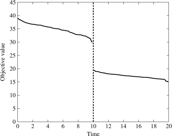
Figure 6.1 Hypothetical objective value obtained through the run for an instance of the DTSP problem.

To assess the quality of the solution independent of the range of the objective values, the following metrics can be considered:

• Error:

  

• Accuracy [31]:

  

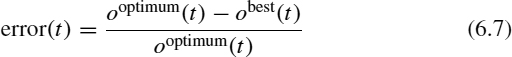
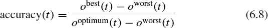
where o^optimum(t) is the objective value of the optimum solution at time t, o^worst(t) is the objective value of the worst solution at time t, and o^best(t) is the objective value of the best solution known at time t. The values of accuracy vary between 0 and 1 on the basis of accuracy (t) = 1 when o^best(t) = o^optimum(t). Additional metrics can be found in the work of Morrison [32] and Weicker [41]. Unfortunately, use of these metrics is not a trivial task for some problems, since it is necessary to know the values for o^optimum(t) and o^worst(t). When these values are not available, a common approach is to use the upper and lower bounds given by the state of the art.

6.5.2 Measuring the Adaptation Cost

Another major goal in dynamic environments is mimimization of the adaptation cost when the scenario has changed (in this situation a decreasing quality of the current solutions is generally observed). To measure the adaptation cost, the following two approaches can be considered: (1) measuring the loss of quality and (2) measuring the time that the algorithm needs to generate solutions of quality similar to that found before the change took place. To do that, Feng et al. [20] propose two metrics:

1. Stability(t), a very important measure in DOPs, which is based on the accuracy values (see Equation 6.8) and is defined as

   

2. -reactivity(t), which denotes the ability of an adaptive algorithm to react quickly to changes and is defined as

   

As with other metrics that measure the solution quality, the metrics above can be represented by curves. However, the stability curve measures the reaction of an MH to changes, and the more common approach (in discrete DOPs) to show the respective values is to consider the average values of stability at the time when changes occur [37].

6.6 CONCLUSIONS

In this chapter we have presented from a unifying point of view a basic set of canonical population-based MHs for DOPs as well as a number of general considerations with respect to the use of adequate benchmarks for DOPs and some standard metrics that can be used to assess MH performance. It is important to note that for specific DOPs and MHs, there exist an important number of implementation details not covered here that should be considered; however, we have given some important suggestions to guide researchers in their work.

Acknowledgments

The first three authors acknowledge funding from the National University of San Luis (UNSL), Argentina and the National Agency for Promotion of Science and Technology, Argentina (ANPCYT). The second author also acknowledges the National Scientific and Technical Research Council (CONICET), Argentina. The fourth author acknowledges funding from the Spanish Ministry of Education and Science and FEDER under contract TIN2005-08818-C04-01 (the OPLINK project).

REFERENCES

1. Y. Abdunnaser. Adapting evolutionary approaches for optimization in dynamic environments. Ph.D. thesis, University of Waterloo, Waterloo, Ontario, Canada, 2006.

2. H. C. Andersen. An investigation into genetic algorithms, and the relationship between speciation and the tracking of optima in dynamic functions. Honours thesis, Queensland University of Technology, Brisbane, Australia, Nov. 1991.

3. P. J. Angeline. Tracking extrema in dynamic environments. In P. J. Angeline, R. G. Reynolds, J. R. McDonnell, and R. Eberhart, eds., Proceedings of the 6th International Conference on Evolutionary Programming (EP'97), Indianapolis, IN, vol. 1213 of Lecture Notes in Computer Science. Springer-Verlag, New York, 1997, pp. 335–345.

4. L. Bianchi. Notes on dynamic vehicle routing: the state of the art. Technical Report IDSIA 05-01. Istituto dalle Mòlle di Studi sull' Intelligènza Artificiale (IDSIA), Manno-Lugano, Switzerland, 2000.

5. T. Blackwell and J. Branke. Multi-swarm optimization in dynamic environments. In G. R. Raidl, S. Cagnoni, J. Branke, D. Corne, R. Drechsler, Y. Jin, C. G. Johnson, P. Machado, E. Marchiori, F. Rothlauf, G. D. Smith, and G. Squillero, eds., Proceedings of Applications of Evolutionary Computing: EvoBIO, EvoCOMNET, EvoHOT, EvoIASP, EvoMUSART, and EvoSTOC (EvoWorkshops'04), vol. 3005 of Lecture Notes in Computer Science. Springer-Verlag, New York, 2004, pp. 489–500.

6. P. A. N. Bosman. Learning, anticipation and time-deception in evolutionary online dynamic optimization. In S. Yang and J. Branke, eds., Proceedings of the 7th Genetic and Evolutionary Computation Conference: Workshop on Evolutionary Algorithms for Dynamic Optimization Problems (GECCO:EvoDOP'05). ACM Press, New York, 2005, pp. 39–47.

7. P. A. N. Bosman and H. La Poutrè. Computationally intelligent online dynamic vehicle routing by explicit load prediction in an evolutionary algorithm. In T. P. Runarsson, H.-G. Beyer, E. Burke, J. J. Merelo-Guervos, and X. Yao, eds., Proceedings of the 9th International Conference on Parallel Problem Solving from Nature (PPSN IX), Reykjavik, Iceland, vol. 4193 of Lecture Notes in Computer Science. Springer-Verlag, New York, 2006, pp. 312–321.

8. P. A. N. Bosman and H. La Poutrè. Learning and anticipation in online dynamic optimization with evolutionary algorithms: the stochastic case. In D. Thierens, ed., Proceedings of the 9th Genetic and Evolutionary Computation Conference (GECCO'07), London. ACM Press, New York, 2007, pp. 1165–1172.

9. J. Branke. Moving peaks benchmark. http://www.aifb.uni-karlsruhe.de-/^~jbr/MovPeaks/movpeaks/.

10. J. Branke. Memory enhanced evolutionary algorithms for changing optimization problems. In P. J. Angeline, Z. Michalewicz, M. Schoenauer, X. Yao, and A. Zalzala, eds., Proceedings of the 1999 IEEE Congress on Evolutionary Computation (CEC'99), Mayflower Hotel, Washington, DC, vol. 3. IEEE Press, Piscataway, NJ, 1999, pp. 1875–1882.

11. J. Branke. Evolutionary Optimization in Dynamic Environments, vol. 3 of On Genetic Algorithms and Evolutionary Computation. Kluwer Academic, Norwell, MA, 2002.

12. J. Branke, T. Kaufler, C. Schmidt, and H. Schmeck. A multipopulation approach to dynamic optimization problems. In I. C. Parmee, ed., Proceedings of the 4th International Conference on Adaptive Computing in Design and Manufacture (ACDM'00), University of Plymouth, Devon, UK., Springer-Verlag, New York, 2000, pp. 299–308.

13. J. Branke and D. Mattfeld. Anticipation in dynamic optimization: the scheduling case. In M. Schoenauer, K. Deb, G. Rudolph, X. Yao, E. Lutton, J. J. Merelo, and H.-P. Schwefel, eds., Proceedings of the 5th International Conference on Parallel Problem Solving from Nature (PPSN V), Inria Hotel, Paris, vol. 1917 of Lecture Notes in Computer Science, Springer-Verlag, New York, 2000, pp. 253–262.

14. W. Cedeno and V. R. Vemuri. On the use of niching for dynamic landscapes. In Proceedings of the International Conference on Evolutionary Computation (ICEC'97), Indianapolis, IN. IEEE Press, Piscataway, NJ, 1997, pp. 361–366.

15. H. G. Cobb. An investigation into the use of hypermutation as an adaptive operator in genetic algorithms having continuous, time-dependent nonstationary environments. Technical Report AIC-90-001. Navy Center for Applied Research in Artificial Intelligence, Washington, DC, 1990.

16. K. A. De Jong. An analysis of the behavior of a class of genetic adaptive systems. Ph.D. thesis, University of Michigan, Ann Arbor, MI, 1975.

17. A. V. Donati, L. M. Gambardella, N. Casagrande, A. E. Rizzoli, and R. Montemanni. Time dependent vehicle routing problem with an ant colony system. Technical Report IDSIA-02-03. Istituto dalle Mòlle Di Studi Sull' Intelligènza Artificiale (IDSIA), Manno-Lugano, Switzerland, 2003.

18. C. J. Eyckelhof and M. Snoek. Ant systems for dynamic problems—the TSP case: ants caught in a traffic jam. In M. Dorigo, G. Di Caro, and M. Sampels, eds., Proceedings of the 3rd International Workshop on Ant Algorithms (ANTS'02), London. vol. 2463 of Lecture Notes in Computer Science. Springer-Verlag, New York, 2002, pp. 88–99.

19. H.-L. Fang, P. Ross, and D. Corne. A promising genetic algorithm approach to job-shop scheduling, re-scheduling, and open-shop scheduling problems. In S. Forrest, ed., Proceedings of the 5th International Conference on Genetic Algorithms (ICGA'93), San Mateo, CA. Morgan Kaufmann, San Francisco, CA, 1993, pp. 375–382.

20. W. Feng, T. Brune, L. Chan, M. Chowdhury, C. K. Kuek, and Y. Li. Benchmarks for testing evolutionary algorithms. Technical Report CSC-97006. Center for System and Control, University of Glasgow, Glasgow, UK, 1997.

21. F. Glover and G. A. Kochenberg, editors. Handbook of Metaheuristics. Kluwer Academic, London, 2003.

22. D. E. Goldberg and R. E. Smith. Nonstationary function optimization using genetic algorithms with dominance and diploidy. In J. J. Grefenstette, ed., Proceedings of the 2nd International Conference on Genetic Algorithms (ICGA'87), Pittsburgh, PA. Lawrence Erlbaum Associates Publishers, Hillsdale, NJ, 1987, pp. 59–68.

23. J. J. Grefenstette. Genetic algorithms for changing environments. In R. Männer and B. Manderickm, eds., Proceedings of the 2nd International Conference on Parallel Problem Solving from Nature (PPSN II), Brussels, Belgium. Elsevier, Amsterdam, 1992, pp. 137–144.

24. M. Guntsch and M. Middendorf. Applying population based ACO to dynamic optimization problems. In M. Dorigo, G. Di Caro, and M. Sampels, eds., Proceedings of the 3rd International Workshop on Ant Algorithms (ANTS'02), London, vol. 2463 of Lecture Notes in Computer Science. Springer-Verlag, New York, 2002, pp. 111–122.

25. M. Guntsch and M. Middendorf. A population based approach for ACO. In S. Cagnoni, J. Gottlieb, E. Hart, M. Middendorf, and G. R. Raidl, eds., Proceedings of Applications of Evolutionary Computing: EvoCOP, EvoIASP, EvoSTIM/EvoPLAN (EvoWorkshops'02), Kinsale, UK, vol. 2279 of Lecture Notes in Computer Science. Springer-Verlag, New York, 2002, pp. 71–80.

26. L. Hongbo and A. Ajith. Fuzzy adaptive turbulent particle swarm optimization. In N. Nedjah, L. M. Mourelle, A. Vellasco, M. M. B. R. and Abraham, and M. Köppen, eds., Proceedings of 5th International Conference on Hybrid Intelligent Systems (HIS'05), Río de Janeiro, Brazil. IEEE Press, Piscataway, NJ, 2005, pp. 445–450.

27. X. Li. Adaptively choosing neighbourhood bests using species in a particle swarm optimizer for multimodal function optimization. In R. Poli et al., eds., Proceedings of the 6th Genetic and Evolutionary Computation Conference (GECCO'04), Seattle, WA, vol. 3102 of Lecture Notes in Computer Science. Springer-Verlag, New York, 2004, pp. 105–116.

28. X. Li, J. Branke, and T. Blackwell. Particle swarm with speciation and adaptation in a dynamic environment. In M. Cattolico, ed., Proceedings of the 8th Genetic and Evolutionary Computation Conference (GECCO'06), Seattle, WA. ACM Press, New York, 2006, pp. 51–58.

29. L. T. Bui, H. A. Abbass, and J. Branke. Multiobjective optimization for dynamic environments. In Proceedings of the 2005 IEEE Congress on Evolutionary Computation (CEC'05), vol. 3, Edinburgh, UK. IEEE Press, Piscataway, NJ, 2005, pp. 2349–2356.

30. R. Mendes and A. Mohais. DynDE: a differential evolution for dynamic optimization problems. In Proceedings of the 2005 IEEE Congress on Evolutionary Computation (CEC'05), Edinburgh, UK. IEEE Press, Piscataway, NJ, 2005, pp. 2808–2815.

31. N. Mori, H. Kita, and Y. Nishikawa. Adaptation to a changing environment by means of the thermodynamical genetic algorithm. In H. Voigt, W. Ebeling, and I. Rechenberg, eds., Proceedings of the 4th International Conference on Parallel Problem Solving from Nature (PPSN IV), Berlin, vol. 1141 of Lecture Notes in Computer Science. Springer-Verlag, New York, 1996, pp. 513–522.

32. R. W. Morrison. Performance measurement in dynamic environments. In E. Cantú-Paz, J. A. Foster, K. Deb, L. Davis, R. Roy, U.-M. O'Reilly, H.-G. Beyer, R. K. Standish, G. Kendall, S. W. Wilson, M. Harman, J. Wegener, D. Dasgupta, M. A. Potter, A. C. Schultz, K. A. Dowsland, N. Jonoska, and J. F. Miller, eds., Proceedings of the 5th Genetic and Evolutionary Computation Conference: Workshop on Evolutionary Algorithms for Dynamic Optimization Problems (GECCO:EvoDOP'03), Chigaco, vol. 2723 of Lecture Notes in Computer Science. Springer-Verlag, New York, 2003, pp. 99–102.

33. R. W. Morrison. Designing Evolutionary Algorithms for Dynamic Environments. Springer-Verlag, New York, 2004.

34. R. W. Morrison and K. A. De Jong. A test problem generator for non-stationary environments. In P. J. Angeline, Z. Michalewicz, M. Schoenauer, X. Yao, and A. Zalzala, eds., Proceedings of the 1999 IEEE Congress on Evolutionary Computation (CEC'99), Mayflower Hotel, Washington, DC, vol. 3. IEEE Press, Piscataway, NJ, 1999, pp. 2047–2053.

35. E. Pettit and K. M. Swigger. An analysis of genetic-based pattern tracking and cognitive-based component tracking models of adaptation. In M. Genesereth, ed., Proceedings of the National Conference on Artificial Intelligence (AAAI'83), Washington, DC. Morgan Kaufmann, San Francisco, CA, 1983, pp. 327–332.

36. H. N. Psaraftis. Dynamic vehicle routing: status and prospect. Annals of Operations Research, 61:143–164, 1995.

37. K. Trojanowski and Z. Michalewicz. Searching for optima in non-stationary environments. In P. J. Angeline, Z. Michalewicz, M. Schoenauer, X. Yao, and A. Zalzala, eds., Proceedings of the 1999 IEEE Congress on Evolutionary Computation (CEC'99), Mayflower Hotel, Washington, DC. IEEE Press, Piscataway, NJ, 1999, pp. 1843–1850.

38. R. K. Ursem. Multinational GA optimization techniques in dynamic environments. In D. Whitley, D. Goldberg, E. Cantú-Paz, L. Spector, I. Parmee, and H.-G. Beyer, eds., Proceedings of the 2nd Genetic and Evolutionary Computation Conference (GECCO'00), Las Vegas, NV. Morgan Kaufmann, San Francisco, CA, 2000, pp. 19–26.

39. J. I. van Hemert and J. A. La Poutrè. Dynamic routing problems with fruitful regions: models and evolutionary computation. In Y. Yao, E. Burke, J. A. Lozano, J. Smith, J. J. Merelo-Guervós, J. A. Bullinaria, J. Rowe, P. , A. Kabán, and H.-P. Schwefel, eds., Proceedings of the 8th International Conference on Parallel Problem Solving from Nature (PPSN VIII), Birmingham, UK, vol. 3242 of Lecture Notes in Computer Science. Springer-Verlag, New York, 2004, pp. 692–701.

40. F. Vavak, K. Jukes, and T. C. Fogarty. Adaptive combustion balancing in multiple burner boiler using a genetic algorithm with variable range of local search. In T. Bäck, ed., Proceedings of the 7th International Conference on Genetic Algorithms (ICGA'97), Michigan State University, East Lansing, MI. Morgan Kaufmann, San Francisco, CA, 1997, pp. 719–726.

41. K. Weicker. Performance measures for dynamic environments. In J. J. Merelo-Guervós, P. Adamidis, H.-G. Beyer, J.-L. Fernández-Villacañas, and H.-P. Schwefel, eds., Proceedings of the 7th International Conference on Parallel Problem Solving from Nature (PPSN VII), Granada, Spain, vol. 2439 of Lecture Notes in Computer Science. Springer-Verlag, New York, 2002, pp. 64–76.

42. D. Zaharie. Control of population diversity and adaptation in differential evolution algorithms. In R. Matousek and P. Osmera, eds., Proceedings of the 9th International Conference of Soft Computing (MENDEL'03), Faculty of Mechanical Engineering, Brno, Czech Republic, June 2003, pp. 41–46.

43. D. Zaharie and F. Zamfirache. Diversity enhancing mechanisms for evolutionary optimization in static and dynamic environments. In Proceedings of the 3rd Romanian–Hungarian Joint Symposium on Applied Computational Intelligence and Informatics (SACI'06), Timisoara, Romania, May 2006, pp. 460–471.