
 CHAPTER 8
Optimization of Time Series Using Parallel, Adaptive, and Neural Techniques
J. A. GÓMEZ, M. D. JARAIZ, M. A. VEGA, and J. M. SÁNCHEZ
Universidad de Extremadura, Spain
8.1 INTRODUCTION
In many science and engineering fields it is necessary to dispose of mathematical models to study the behavior of phenomena and systems whose mathematical description is not available a priori. One interesting type of such systems is the time series (TS). Time series are used to describe behavior in many fields: astrophysics, meteorology, economy, and so on. Although the behavior of any of these processes may be due to the influence of several causes, in many cases the lack of knowledge of all the circumstances makes it necessary to study the process considering only the TS evolution that represents it. Therefore, numerous methods of TS analysis and mathematical modeling have been developed. Thus, when dealing with TS, all that is available is a signal under observation, and the physical structure of the process is not known. This led us to employ planning system identification (SI) techniques to obtain the TS model. With this model a prediction can be made, but taking into account that the model precision depends on the values assigned to certain parameters.
The chapter is structured as follows. In Section 8.2 we present the necessary background on TS and SI. The problem is described in Section 8.3, where we have focused the effort of analysis on a type of TS: the sunspot (solar) series. In Section 8.4 we propose a parallel and adaptive heuristic to optimize the identification of TS through adjusting the SI main parameters with the aim of improving the precision of the parametric model of the series considered. This methodology could be very useful when the high-precision mathematical modeling of dynamic complex systems is required. After explaining the proposed heuristics and the tuning of their parameters, in Section 8.5 we show the results we have found for several series using different implementations and demonstrate how the precision improves.
8.2 TIME SERIES IDENTIFICATION
SI techniques [1,2] can be used to obtain the TS model. The model precision depends on the values assigned to certain parameters. In SI, a TS is considered as a sampled signal y(k) with period T that is modeled with an ARMAX [3] polynomial description of dimension na (the model size), as we can see:
Basically, the identification consists of determining the ARMAX model parameters ai (θ in matrix notation) from measured samples y(ki) [ϕ(k) in matrix notation]. In this way it is possible to compute the estimated signal ye(k)
and compare it with the real signal y(k), calculating the generated error:
The recursive estimation updates the model (ai) in each time step k, thus modeling the system. The greater number of sample data that are processed, the more precise the model because it has more system behavior history. We consider SI performed by the well-known recursive least squares (RLS) algorithm [3]. This algorithm is specified primarily by the forgetting factor constant λ and the samples observed, y(k). There is no fixed value for λ; a value between 0.97 and 0.995 is often used [4]. From a set of initial conditions [k = p, θ(p) = 0, P(p) = 1000I, where I is the identity matrix and p is the initial time greater than the model size na], RLS starts building ϕT(k), doing a loop of operations defined in Equations 8.2 to 8.6.


The recursive identification is very useful when it is a matter of predicting the following behavior of the TS from the data observed up to the moment. For many purposes it is necessary to make this prediction, and for predicting it is necessary to obtain information about the system. This information, acquired by means of the SI, consists in elaborating a mathematical parametric model to cover system behavior.

Figure 8.1 Sunspot series used as a benchmark to evaluate the algorithmic proposal.
We use a TS set as benchmark to validate the algorithmic proposal that we present in this chapter. Some of these benchmarks have been collected from various processes [5] and others correspond to sunspot series acquired from measured observations of the sun activity [6,7]. For this type of TS we have used 13 series (Figure 8.1) showing daily sunspots: 10 series (ss_00, ss_10, ss_20, ss_30, ss_40, ss_50, ss_60, ss_70, ss_80, and ss_90) corresponding to sunspot measurements covering 10 years each (e.g., ss_20 compiles the sunspots from 1920 to 1930), two series (ss_00_40 and ss_50_90) covering 50 years each, and one series (ss_00_90) covering all measurements in the twentieth century.
8.3 OPTIMIZATION PROBLEM
When SI techniques are used, the model is generated a posteriori by means of the data measured. However, we are interested in system behavior prediction in running time, that is, while the system is working and the data are being observed. So it would be interesting to generate models in running time in such a way that a processor may simulate the next behavior of the system. At the same time, our first effort is to obtain high model precision. SI precision is due to several causes, mainly to the forgetting factor (Figure 8.2). Frequently, this value is critical for model precision. Other sources can also have some degree of influence (dimensions, initial values, the system, etc.), but they are considered as problem definitions, not parameters to be optimized. On the other hand, the precision problem may appear when a system model is generated in sample time for some dynamic systems: If the system response changes quickly, the sample frequency must be high to avoid the key data loss in the system behavior description. If the system is complex and its simulation from the model to be found must be very trustworthy, the precision required must be very high, and this implies a great computational cost. Therefore, we must find a trade-off between high sample frequency and high precision in the algorithm computation. However, for the solar series, the interval of sampling is not important, the real goal being to obtain the maximum accuracy of estimation.
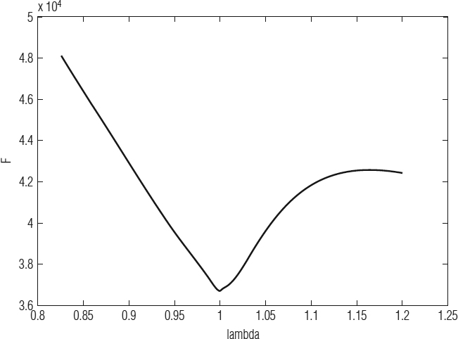
Figure 8.2 Error in identification for several λ values using RLS for ss_80 benchmark when na = 5. It can be seen that the minimum error is reached when λ = 0.999429.
Summarizing, the optimization problem consists basically of finding the λ value such that the identification error is minimum. Thus, the fitness function F,
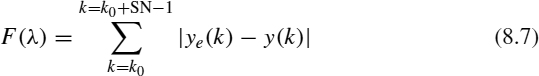
is defined as the value to minimize to obtain the best precision, where SN is the number of samples. The recursive identification can be used to predict the behavior of the TS [Figure 8.3(a)] from the data observed up to the moment. It is possible to predict system behavior in k + 1, k + 2, … by means of the model θ(k) identified in k time. As identification advances in time, the predictions improve, using more precise models. If ks is the time until the model is elaborated and for which we carry out the prediction, we can confirm that this prediction will have a larger error while we will be farther away from ks [Figure 8.3(b)]. The value predicted for ks + 1 corresponds to the last value estimated until ks. When we have more data, the model starts to be reelaborated for computing the new estimated values [Figure 8.3(c)].
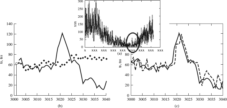
Figure 8.3 (a) The ss_90 series. If ks = 3000, we can see in (b) the long-term prediction based on the model obtained up to ks (na = 30 and λ = 0.98). The prediction precision is reduced when we are far from ks. (c) Values predicted for the successive ks + 1 obtained from the updated models when the identification (and ks) advances.
The main parameters of the identification are na and λ. Both parameters have an influence on the precision of prediction results, as shown in Figures 8.4 and 8.5. As we can see, establishing an adequate value of na and λ may be critical in obtaining a high-quality prediction. Therefore, in the strategy to optimize the prediction we try, first, to establish a satisfactory dimension of the mathematical model (i.e., a model size giving us good results without too much computational cost), which will serve us later in finding the optimal λ value (the optimization problem). To do that, many experiments have been carried out. In these experiments the absolute difference between the real and predicted values has been used to quantify the prediction precision. Fitness in the prediction experiments is measured as
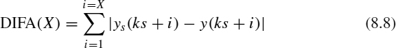
We use our own terminology for the prediction error [DIFA(X), where X is an integer], allowing the reader to understand more easily the degree of accuracy that we are measuring. Figure 8.6 shows the results of many experiments, where different measurements of the prediction error [for short-term DIFA(1) and for long-term DIFA(50)] for 200 values of the model size are obtained. These experiments have been made for different ks values to establish reliable conclusions.
For the experiments made we conclude that the increase in model size does not imply an improvement in the prediction precision (however, a considerable increase in computational cost is achieved). This is easily verified using large ks values (the models elaborated have more information related to the TS) and long-term predictions. From these results and as a trade-off between prediction and computational cost, we have chosen na = 40 to fix the model size for future experiments.
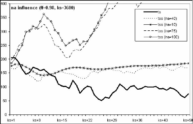
Figure 8.4 Influence of the model size na on short-term (ks) and long-term (ks + 50) prediction for the ss_90 series.

Figure 8.5 Influence of the forgetting factor λ on short-term (ks) and long-term (ks + 50) prediction for the ss_90 series.

Figure 8.6 Precision of the prediction for the ss_90 series from ks = 3600 using λ = 0.98. The measurements have been made for models with sizes between 2 and 200.
The forgetting factor is the key parameter for prediction optimization. Figure 8.7 shows, with more detail than Figure 8.3(b), an example of the λ influence on the short- and long-term predictions by means of the representation of the measurement of its precision. It is clear that for any λ value, short-term prediction is more precise than long-term prediction. However, we see that the value chosen for λ is critical to finding a good predictive model (from the four values chosen, λ = 1 produces the prediction with minimum error, even in the long term). This analysis has been confirmed by carrying out a great number of experiments with the sunspot series, modifying the initial prediction time ks.

Figure 8.7 Influence of λ in the prediction precision for ss_90 with na = 40 and ks = 3600
8.4 ALGORITHMIC PROPOSAL
To find the optimum value of λ, we propose a parallel adaptive algorithm that is partially inspired by the concept of artificial evolution [8,9] and the simulated annealing mechanism [10]. In our proposed PARLS (parallel adaptive recursive least squares) algorithm, the optimization parameter λ is evolved for predicting new situations during iterations of the algorithm. In other words, λ evolves, improving its fitness.
The evolution mechanism (Figure 8.8) is as follows. In its first iteration, the algorithm starts building a set of λ values (individuals in the initial population) covering the interval R (where the individuals are generated) uniformly from the middle value selected (λc). Thus, we assume that the population size is the length R, not the number of individuals in the population. A number of parallel processing units (PUN) equal to the number of individuals perform RLS identification with each λ in the population. Therefore, each parallel processing unit is an identification loop that considers a given number of samples (PHS) and an individual in the population as the forgetting factor. At the end of the iteration, the best individual is the one whose corresponding fitness has the minimum value of all those computed in the parallel processing units, and from it a new set of λ values (the new population) is generated and used in the next iteration to perform new identifications during the following PHS samples.
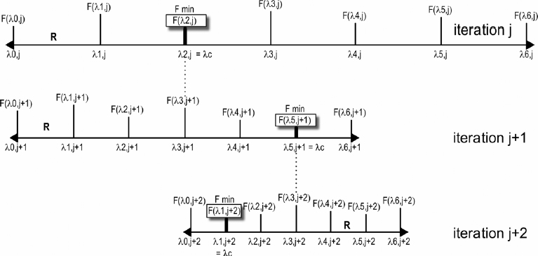
Figure 8.8 For an iteration of the algorithm, the individuals λ of the population are the inputs for RLS identifications performed in parallel processing units. At the end of iteration the best individual is the one whose fitness F is minimal, and from it a new population is generated covering a more reduced interval.
Fitness F is defined as the accumulated error of the samples in the iteration according to Equation 8.7:

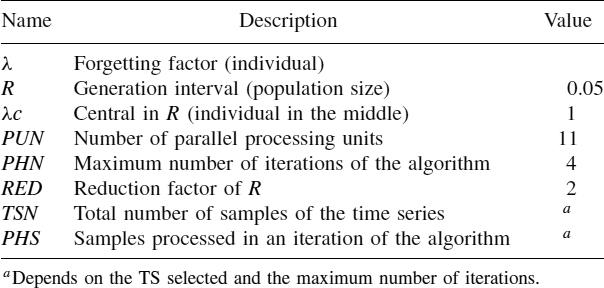
Generation of the new population is made with a more reduced interval, dividing R by a reduction factor (RED). In this way the interval limits are moved so that the middle of the interval corresponds to the best found individual in the preceding iteration, such way that the population generated will be nearer the previous best individual found. The individuals of the new population always cover the new interval R uniformly. Finally, PARLS stops when the maximum number of iterations (PHN) is reached, according to the total number of samples (TSN) of the TS or when a given stop criterion is achieved. PARLS nomenclature is summarized in Table 8.1, and pseudocode of this algorithmic proposal is given in Algorithm 8.1
TABLE 8.1 PARLS Nomenclature and Tuned Values
Algorithm 8.1 Parallel Adaptive Algorithm

The goal of the iterations of the algorithm is that the identifications performed by the processing units will converge to optimum λ values, so the final TS model will be of high precision. Therefore, PARLS could be considered as a population-based metaheuristic rather than a parallel metaheuristic, because each processing unit is able to operate in isolation, as well as the relevant problem itself, as only a single real-valued parameter (λ) is optimized.
Each processing unit performs the RLS algorithm as it is described in Equations 8.2 to 8.6. NNPARLS is the PARLS implementation, where the parallel processing units are built by means of neural networks [11]. With this purpose we have used the NNSYSID toolbox [12] of Matlab [13]. In this toolbox the multilayer perceptron network is used [14] because of its ability to model any case. For this neural net it is necessary to fix several parameters: general architecture (number of nodes), stop criterion (the training of the net is concluded when the stop criterion is lower than a determined value), maximum number of iterations (variable in our experiments), input to hidden layer and hidden to output layer weights, and others.
8.5 EXPERIMENTAL ANALYSIS
PARLS offers great variability for their parameters. All the parameters have been fully checked and tested in order to get a set of their best values, carrying out many experiments with a wide set of benchmarks. According to the results we have obtained, we can conclude that there are not common policies to tune the parameters in such a way that the best possible results will always be found. But the experiments indicate that there is a set of values of the main parameters for which the optimal individual found defines an error in the identification less than the one obtained with classical or randomly chosen forgetting factor values. We can establish fixed values for PARLS parameters (the right column in Table 8.1) to define a unique algorithm implementation easily applicable to any TS. This has the advantage of a quick application for a series without the previous task of tuning parameters.
A question of interest relates to the adequate model size. There is a large computational cost in time when na is high, as we can see in Figure 8.9. Therefore, the model size should be selected in relation to the computational cost required, and this size is considered as part of the definition of the problem, not as part of the optimization heuristic. We have computed several series with different values for na with processing units implemented with neural networks. Our conclusion is that an accurate tuning for general purposes could be from na = 20, although this value can be increased considerably for systems with wide sampling periods. Since a larger na value increases the model precision, for the sunspot series an adequate value of na can be 40, since the time required to compute is tolerable because the series has a long sampling interval (one day).
Another important question relates to how to establish the initial population by selecting the limits of the valid range. We have performed lots of experiments to determine the approximate optimal individual for several TSs using massive RLS computations. Some of these experiments are shown in Figure 8.10. We can see that there is a different best solution for each TS, but in all cases there is a smooth V-curve that is very useful in establishing the limits of the initial population. We have selected the tuned values λc = 1 and R = 0.05, from which we can generate the initial population. Observing the results, it could be said that the optimum value is λ = 1, but it is dangerous to affirm this if we have not reduced the range more. Then, by reducing the interval of search we will be able to find a close but different optimum value than 1, as we can see in Figure 8.11.

Figure 8.9 Increment of the computation time with model size for the kobe benchmark using a Pentium-41.7 GHz–based workstation, evaluating 101 or 201 values of the forgetting factor.
In Figure 8.12 compare the results of an RLS search and the PARLS algorithm for several sunspot series. In all cases the same tuned parameters have been used (na = 20, PUN = 11, λc = 1, R = 0.05, RED = 2, PHN = 4). The computational effort of 11 RLS identifications is almost equal to PARLS with 11 processing units, so the results can be compared to establish valid conclusions. With these tuned parameters, PARLS always yields better results than RLS. This fact contrasts with the results obtained for other types of TSs, for which PARLS yields better results in most, but for a few TSs the difference in the corresponding fitness oscillates between 2 and 5% in favor of RLS. Therefore, if for the series studied we said that PARLS improves or holds the results found by RLS using the same computational effort, for the sunspot solar series we can say that PARLS always gives us better results [15].
Due to the fact that PARLS has obtained good results, we believe that it can be useful for prediction purposes. In this way we have computed some experiments to predict the next values from the last value registered for sun activity in the second half of the twentieth century. The results are shown in Figure 8.13. Prediction precision is given by the measurements DIFA(1) (short term) and DIFA(50) (long term). These results are compared, for evaluation purposes, with those obtained using RLS identification with some values of λ inside the classic range [4]. It can be seen that PARLS yields better precision.
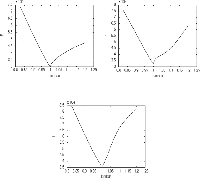
Figure 8.10 Fitness of the sunspot series ss_10, ss_20, and ss_40, calculated by RLS for 200 λ values in the same range (λc = 1, R = 0.4) using the same model size (na = 20). We can see a smooth V-curve in all the cases.

Figure 8.11 Fitness of the ss_90 series calculated by RLS for 100 λ values in two different ranges (R = 0.4 and R = 0.002), both centered in λc = 1 and using the same model size (na = 20). It can be seen that the optimal λ value is not 1, and how it can be found by using a narrower range.
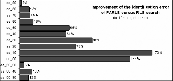
Figure 8.12 Review of some results. This figure shows a comparison of results between an RLS search (where each RLS execution searches the best fitness among 11 values of λ) and PARLS for several series with the same tuned parameters. The Minimum error was always found for the PARLS algorithm for all the series.
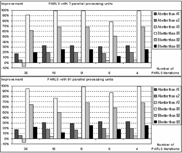
Figure 8.13 Sample of the precision of for short- and long-term prediction results compared with those obtained from three classical values of λ: 0.97, 0.98, and 0.995. A and B are DIFA1 and DIFA50 for λopt, respectively. A1 and B1 are DIFA1 and DIFA50 for λ = 0.97, A2 and B2 are DIFA1 and DIFA50 for λ = 0.98, and A3 and B3 are DIFA1 and DIFA50 for λ = 0.995. The settings for these experiment were: benchmark ss_50_90; na = 40; ks = 18,210; TSN = 18,262; λc = 1; R = 0.2; RED = 2. PARLS uses the tuned values of its paremeters in Table 8.1, where the processing units were implemented with neural networks.
8.6 CONCLUSIONS
As a starting point, we can say that the parallel adaptive algorithm proposed offers a good performance, and this encourages us to follow this research. The results shown in Section 8.5 are part of a great number of experiments carried out using different TS and initial prediction times. In the great majority of the cases, PARLS offers a smaller error in the identification than if λ random values are used. Also, the neural network implementation of the parallel processing units has offered better results than in conventional programming [11]. However, we are trying to increase the prediction precision. Thus, our future working lines suggest using genetic algorithms or strategies of an analogous nature, on the one hand, to find the optimum set of values for the parameters of PARLS, and on the other hand, to find the optimum pair of values {na, λ} (in other words, to consider the model size as an optimization parameter; in this case, multiobjective heuristics are required).
Acknowledgments
The authors are partially supported by the Spanish MEC and FEDER under contract TIC2002-04498-C05-01 (the TRACER project).
REFERENCES
1. T. Soderstrom. System Identification. Prentice-Hall, Englewood Cliffs, NJ, 1989.
2. J. Juang. Applied System Identification. Prentice Hall, Upper Saddle River, NJ, 1994.
3. L. Ljung. System Identification. Prentice Hall, Upper Saddle River, NJ, 1999.
4. L. Ljung. System Identification Toolbox. MathWorks, Natick, MA, 1991.
5. I. Markovsky, J. Willems, and B. Moor A database for identification of systems. In Proceedings of the 17th International Symposium on Mathematical Theory of Networks and Systems, 2005, pp. 2858–2869.
6. P. Vanlommel, P. Cugnon, R. Van Der Linden, D. Berghmans, F. Clette. The Sidc: World Data Center for the Sunspot Index. Solar Physics 224:113–120, 2004.
7. Review of NOAA s National Geophysical Data Center. National Academies Press, Washington, DC, 2003.
8. D. Goldberg. Genetic Algorithms in Search, Optimization and Machine Learning. Addison-Wesley, Reading, MA, 1989.
9. D. Fogel. Evolutionary Computation: Toward a New Philosophy of Machine Intelligence. IEEE Press, Piscataway, NJ, 2006.
10. S. Kirkpatrick, C. Gelatt, and M. Vecchi. Optimization by simulated annealing. Science, 220:671–680, 1983.
11. J. Gomez, J. Sanchez, and M. Vega. Using neural networks in a parallel adaptive algorithm for the system identification optimization. Lecture Notes in Computer Science, 2687:465–472, 2003.
12. M. Nørgaard. System identification and control with neural networks. Ph.D. thesis, Department of Automation, University of Denmark, 1996.
13. R. Pratap. Getting Started with Matlab. Oxford University Press, New York, 2005.
14. H. Demuth and M. Beale. Neural Network Toolbox. MathWorks, Natick, MA, 1993.
15. J. Gomez, M. Vega, and J. Sanchez. Parametric identification of solar series based on an adaptive parallel methodology. Journal of Astrophysics and Astronomy, 26:1–13, 2005.
Optimization Techniques for Solving Complex Problems, Edited by Enrique Alba, Christian Blum, Pedro Isasi, Coromoto León, and Juan Antonio Gómez
Copyright © 2009 John Wiley & Sons, Inc.