CHAPTER 23

Solving the KCT Problem: Large-Scale Neighborhood Search and Solution Merging

C. BLUM and M. J. BLESA

Universitat Politècnica de Catalunya, Spain

23.1 INTRODUCTION

In recent years, the development of hybrid metaheuristics for optimization has become very popular. A hybrid metaheuristic is obtained by combining a metaheuristic intelligently with other techniques for optimization: for example, with complete techniques such as branch and bound or dynamic programming. In general, hybrid metaheuristics can be classified as either collaborative combinations or integrative combinations. Collaborative combinations are based on the exchange of information between a metaheuristic and another optimization technique running sequentially (or in parallel). Integrative combinations utilize other optimization techniques as subordinate parts of a metaheuristic. In this chapter we present two integrative combinations for tackling the k-cardinality tree (KCT) problem. The hybridization techniques that we use are known as large-scale neighborhood search and solution merging. The two concepts are related. In large-scale neighborhood search, a complete technique is used to search the large neighborhood of a solution to find the best neighbor. Solution merging is known from the field of evolutionary algorithms, where the union of two (or more) solutions is explored by a complete algorithm to find the best possible offspring solution. We refer the interested reader to the book by Blum et al. [5] for a comprehensive introduction to hybrid metaheuristics.

23.1.1 Background

The k-cardinality tree (KCT) problem was defined by Hamacher et al. [23]. Subsequently [17,26], the NP-hardness of the problem was shown. The problem has several applications in practice (see Table 23.1).

TABLE 23.1 Applications of the KCT Problem

Application	References
Oil-field leasing	[22]
Facility layout	[18,19]
Open-pit mining	[27]
Matrix decomposition	[8,9]
Quorum-cast routing	[12]
Telecommunications	[21]

Technically, the KCT problem can be described as follows. Let G(V,E) be an undirected graph in which each edge e ∈ E has a weight w_e ≥ 0 and each node υ ∈ V has a weight w_υ ≥ 0. Furthermore, we denote by the set of all k-cardinality trees in G, that is, the set of all trees in G with exactly k edges. The problem consists of finding a k-cardinality tree T_k ∈ that minimizes

Henceforth, when given a tree T, E_T denotes the set of edges of T and V_T the set of nodes of T.

23.1.2 Literature Review

The literature treats mainly two special cases of the general KCT problem as defined above: (1) the edge-weighted KCT (eKCT) problem, where all node weights are equal to zero, and (2) the node-weighted KCT (nKCT) problem, where all edge weights are equal to zero. The eKCT problem was first tackled by complete techniques [12,20,28] and heuristics [12,15,16]. The best working heuristics build (in some way) a spanning tree of the given graph and subsequently apply a polynomial time dynamic programming algorithm [25] that finds the best k-cardinality tree in the given spanning tree. Later, research focused on the development of metaheuristics [6,11,29].

Much less research effort was directed at the nKCT problem. Simple greedy- as well as dual greedy-based heuristics were proposed in [16]. The first metaheuristic approaches appeared in [7,10].

23.1.3 Organization

The organization of this chapter is as follows. In Section 23.2 we outline the main ideas of two hybrid metaheuristics for the general KCT problem. First, we deal with an ant colony optimization (ACO) algorithm that uses large-scale neighborhood search as a hybridization concept. Subsequently, we present the main ideas of an evolutionary algorithm (EA) that uses a recombination operator based on solution merging. Finally, we present a computational comparison of the two approaches with state-of-the-art algorithms from the literature. The chapter finishes with conclusions.

23.2 HYBRID ALGORITHMS FOR THE KCT PROBLEM

The hybrid algorithms presented in this work have some algorithmic parts in common. In the following we first outline these common concepts, then specify the metaheuristics.

23.2.1 Common Algorithmic Components

First, both algorithms that we present are based strongly on tree construction, which is well defined by the definition of the following four components:

1. The graph G′ = (V′,E′) in which the tree should be constructed (here G′ is a subgraph of a given graph G)
2. The required size l ≤ (V′ − 1) of the tree to be constructed, that is, the number of required edges the tree should contain
3. The way in which to begin tree construction (e.g., by determining a node or an edge from which to start the construction process)
4. The way in which to perform each construction step

The first three aspects are operator dependent. For example, our ACO algorithm will use tree constructions that start from a randomly chosen edge, whereas the crossover operator of the EA starts a tree construction from a partial tree. However, the way in which to perform a construction step is the same in all tree constructions used in this chapter: Given a graph G′ = (V′, E′), the desired size l of the final tree, and the current tree T whose size is smaller than l, a construction step consists of adding exactly one node and one edge to T such that the result is again a tree. At an arbitrary construction step, let (where ) be the set of nodes of G′ that can be added to T via at least one edge. (Remember that V_T denotes the node set of T.) For each υ ∈ , let E_υ be the set of edges that have υ as an endpoint and that have their other endpoint, denoted by υ_e,o, in T. To perform a construction step, a node υ ∈ must be chosen. This can be done in different ways. In addition to the chosen node υ, the edge that minimizes

is added to the tree. For an example, see Figure 23.1.

Second, both algorithms make use of a dynamic programming algorithm for finding the best k-cardinality tree in a graph that is itself a tree. This algorithm, which is based on the ideas of Maffioli [25], was presented by Blum [3] for the general KCT problem.

Figure 23.1 Graph with six nodes and eight edges. For simplicity, the node weights are all set to 1. Nodes and edges are labeled with their weights. Furthermore, we have given a tree T of size 2, denoted by shaded nodes and bold edges: V_T = {υ₁, υ₂, υ₃}, and E_T = {e_1,2, e_1,3}. The set of nodes that can be added to T is therefore given as = {υ₄, υ₅}. The set of edges that join υ₄ with T is E_υ4 = {e_2,4, e_3,4}, and the set of edges that join υ₅ with T is E_υ5 = {e_3,5}. Due to the edge weights, e_min in the case of υ₄ is determined as e_2,4, and in the case of υ₅, as e_3,5.

23.2.2 ACO Combined with Large-Scale Neighborhood Search

ACO [13,14] emerged in the early 1990s as a nature-inspired metaheuristic for the solution of combinatorial optimization problems. The inspiring source of ACO is the foraging behavior of real ants. When searching for food, ants initially explore the area surrounding their nest in a random manner. As soon as an ant finds a food source, it carries to the nest some of the food found. During the return trip, the ant deposits a chemical pheromone trail on the ground. The quantity of pheromone deposited, which may depend on the quantity and quality of the food, will guide other ants to the food source. The indirect communication established via the pheromone trails allows the ants to find the shortest paths between their nest and food sources. This behavior of real ants in nature is exploited in ACO to solve discrete optimization problems using artificial ant colonies.

The hybridization idea of our implementation for the KCT problem is as follows. At each iteration, n_a artificial ants each construct a tree. However, instead of stopping the tree construction when cardinality k is reached, the ants continue constructing until a tree of size l > k is achieved. To each of these l-cardinality trees is then applied Blum's dynamic programming algorithm [3] to find the best k-cardinality tree in this l-cardinality tree. This can be seen as a form of large-scale neighborhood search. The pheromone model used by our ACO algorithm contains a pheromone value τ_e for each edge e ∈ E. After initialization of the variables (i.e., the best-so-far solution), (i.e., the restart-best solution), and cf (i.e., the convergence factor), all the pheromone values are set to 0.5. At each iteration, after generating the corresponding trees, some of these solutions are used to update the pheromone values. The details of the algorithmic framework shown in Algorithm 23.1 are explained in the following.

Algorithm 23.1 Hybrid ACO for the KCT Problem (HyACO)

ConstructTree(,l) The construction of a tree works as explained in Section 23.2.1. It only remains to specify (1) how to start a tree construction, and (2) how to use the pheromone model for choosing among the nodes (and edges) that can be added to the current tree at each construction step. Each tree construction starts from an edge e = (υ_i, υ_j) that is chosen probabilistically in proportion to the values τ_e/(w_e + w_υi + w_υj). With probability , an ant chooses the node υ ∈ that minimizes τ_e · (w_emin + w_υ). Otherwise, υ is chosen probabilistically in proportion to τ_e · (w_emin + w_υ). Two parameters have to be fixed: the probability that determines the percentage of deterministic steps during the tree construction, and l, the size of the trees constructed by the ants. After tuning, we chose the setting for the application to node-weighted grid graphs, and the setting for the application to edge-weighted graphs, where s = (|V| − 1 − k)/4. The tuning process has been outlined in detail by Blum and Blesa [4].

LargeScaleNeighborhoodSearch This procedure applies the dynamic programming algorithm [3] to an l-cardinality tree (where j denotes the tree constructed by the jth ant). The algorithm returns the best k-cardinality tree embedded in .

Update In this procedure, and are set to (i.e., the iteration-best solution) if and , respectively.

ApplyPheromoneUpdate(cf, bs_update, , , , ) As described by Blum and Blesa [6] for a standard ACO algorithm, the HyACO algorithm may use three different solutions for updating the pheromone values: (1) the restart-best solution , (2) the restart-best solution , and (3) the best-so-far solution . Their influence depends on the convergence factor cf, which provides an estimate about the state of convergence of the system. To perform the update, first an update value ξ_e for every pheromone trail parameter is computed:

where κ_ib is the weight of , κ_rb the weight of , and κ_bs the weight of such that κ_ib + κ_rb + κ_bs = 1.0. The δ-function is the characteristic function of the set of edges in the tree; that is, for each k-cardinality tree T_k,

Then the following update rule is applied to all pheromone values τ_e:

where ρ ∈ (0, 1] is the evaporation (or learning) rate. The upper and lower bounds τ_max = 0.99 and τ_min = 0.01 keep the pheromone values in the range (τ_min, τ_max), thus preventing the algorithm from converging to a solution. After tuning, the values for ρ, κ_ib, κ_rb, and κ_bs are chosen as shown in Table 23.2.

TABLE 23.2 Schedule Used for Values ρ, κ_ib, κ_rb, and κ_bs Depending on cf (the Convergence Factor) and the Boolean Control Variable bs_update

ComputeConvergenceFactor This function computes, at each iteration, the convergence factor as

where τ_max is again the upper limit for the pheromone values. The convergence factor cf can therefore only assume values between 0 and 1. The closer cf is to 1, the higher is the probability to produce the solution .

23.2.3 Evolutionary Algorithm Based on Solution Merging

Evolutionary algorithms (EAs) [1,24] are used to tackle hard optimization problems. They are inspired by nature's capability to evolve living beings that are well adapted to their environment. EAs can be characterized briefly as computational models of evolutionary processes working on populations of individuals. Individuals are in most cases solutions to the tackled problem. EAs apply genetic operators such as recombination and/or mutation operators in order to generate new solutions at each iteration. The driving force in EAs is the selection of individuals based on their fitness. Individuals with higher fitness have a higher probability to be chosen as members of the next iteration's population (or as parents for producing new individuals). This principle is called survival of the fittest in natural evolution. It is the capability of nature to adapt itself to a changing environment that gave the inspiration for EAs.

The algorithmic framework of our hybrid EA approach to tackle the KCT problem is shown in Algorithm 23.2. In this algorithm, henceforth denoted by HyEA, T_k^best denotes the best solution (i.e., the best k-cardinality tree) found since the start of the algorithm, and T_k^iter denotes the best solution in the current population P. The algorithm begins by generating the initial population in the function GenerateInitialPopulation(pop_size). Then at each iteration the algorithm produces a new population by first applying a crossover operator in the function ApplyCrossover(P), and then by subsequent replacement of the worst solutions with newly generated trees in the function IntroduceNewMaterial (). The components of this algorithm are outlined in more detail below.

Algorithm 23.2 Hybrid EA for the KCT Problem (HyEA)

GenerateInitialPopulation (pop-size) The initial population is generated in this method. It takes as input the size pop_size of the population, which was set depending on the graph size and the desired cardinality:

The construction of each of the initial k-cardinality trees in graph G begins with a node that is chosen uniformly at random from V. At each further construction step is chosen, with probability , the node υ that minimizes w_emin + w_υ (see also Section 23.2.1). Otherwise (i.e., with probability ), υ is chosen probabilistically in proportion to w_emin + w_υ. Note that when is close to 1, the tree construction is almost deterministic, and the other way around. After tuning by hand (see ref. 2 for more details) we chose for each tree construction a uniform value for from [0.85, 0.99].

ApplyCrossover(P) At each algorithm iteration an offspring population is generated from the current population P. For each k-cardinality tree T ∈ P, the following is done. First, tournament selection (with tournament size 3) is used to choose a crossover partner T^c ≠ T for T from P. In the following we say that two trees in the same graph are overlapping if and only if they have at least one node in common. In case T and T^c are overlapping, graph G^c is defined as the union of T and T^c; that is, V_G^c = V_T ∪ V_T^c and E_G^c = E_T ∪ E_T^c. Then a spanning tree T^sp of G^c is constructed as follows. The first node is chosen uniformly at random. Each further construction step is performed as described above (generation of the initial population). Then the dynamic programming algorithm [3] is applied to T^sp for finding the best k-cardinality tree T^child that is contained in T^sp. Otherwise, that is, in case the crossover partners T and T^c are not overlapping, T is used as the basis for constructing a tree in G that contains both, T and T^c. This is done by extending T (with construction steps as outlined in Section 23.2.1) until the current tree under construction can be connected with T^c by at least one edge. In the case of several connecting edges, the edge e = (υ_i, υ_j) that minimizes w_e + w_υi + w_υj is chosen. Finally, we apply the dynamic programming algorithm [3] for finding the best k-cardinality tree T^child in the tree constructed. The better tree among T^child and T is added to the offspring population . Finally, note that both crossover cases can be seen as implementations of the solution merging concept.

IntroduceNewMaterial To avoid premature convergence of the algorithm, at each iteration this function introduces new material (in the form of newly constructed k-cardinality trees) into the population. The input of this function is the offspring population generated by crossover. First, the function selects of the best solutions in for the new population P. Then the remaining 100 − X% of P are generated as follows: Starting from a node of G that is chosen uniformly at random, an l_new-cardinality tree T_lnew (where l_new ≥ k) is constructed by applying construction steps as outlined above. Here we chose

and newmat = 20 (see ref. 2 for details). Then the dynamic programming algorithm [3] is used to find the best k-cardinality tree in T_lnew. This tree is then added to P.

23.3 EXPERIMENTAL ANALYSIS

We implemented both HyACO and HyEA in ANSI C++ using GCC 3.2.2 to compile the software. Our experimental results were obtained on a PC with Intel Pentium-4 processor (3.06 GHz) and 1 Gb of memory.

23.3.1 Application to Node-Weighted Grid Graphs

First, we applied HyACO and HyEA to the benchmark set of node-weighted grid graphs that was proposed in [10]. This set is composed of 30 grid graphs, that is, 10 grid graphs of 900 vertices (i.e., 30 times 30 vertices), 10 grid graphs of 1600 vertices, and 10 grid graphs of 2500 vertices. We compared our results to the results of the variable neighborhood decomposition search (denoted by VNDS) presented by Brimberg et al. [10]. This comparison is shown in Table 23.3. Instead of applying an algorithm several times to the same graph and cardinality, it is general practice for this benchmark set to apply the algorithm exactly once to each graph and cardinality, and then to average the results over graphs of the same type. The structure of Table 23.3 is as follows. The first table column indicates the graph type (e.g., grid graphs of size 30 × 30), the second column contains the cardinality, and the third table column provides the best known results (abbreviated as bkr). A best-known result is marked with a left–right arrow in case it was produced by one of our algorithms. Then for each of the three algorithms we provide the result (as described above) together with the average computation time that was spent to compute this result. Note that the computation time limit for HyACO and HyEA was approximately the same as the one that was used for VNDS [10]. The computer used to run the experiments [10] is about seven times slower than the machine we used. Therefore, we divided the computation time limits of VNDS by 7 to obtain our computation time limits.

Concerning the results, we note that in 9 out of 15 cases both HyACO and HyEA are better than VNDS. It is interesting to note that this concerns especially small to medium-sized cardinalities. For larger cardinalities, VNDS beats both HyACO and HyEA. Furthermore, HyEA is in 11 out of 15 cases better than HyACO. This indicates that even though HyACO and HyEA behave similarly to VNDS, HyEA seems to make better use of the dynamic programming algorithm than does HyACO. The computation times of the algorithms are of the same order of magnitude.

23.3.2 Application to Edge-Weighted Random Graphs

We also applied HyACO and HyEA to some of the edge-weighted random graph instances from ref. 29 (i.e., 10 instances with 1000, 2000, and 3000 nodes, respectively). The results are shown in Table 23.4 compared to the VNDS algorithm presented by et al. [29]. Note that this VNDS is the current state-of-the-art algorithm for these instances. (The VNDS algorithms for node- and edge-weighted graphs are not the same. They are specialized for the corresponding special cases of the KCT problem.) The machine that was used to run VNDS is about 10 times slower than our machine. Therefore, we used as time limits for HyACO and HyEA one-tenth of the time limits of VNDS.

In general, the results show that the performance of all three algorithms is very similar. However, in 6 out of 15 cases our algorithms (together) improve over the performance of VNDS. Again, the advantage of our algorithms is for small and medium-sized cardinalities. This advantage drops when the size of the graphs increases. Comparing HyACO with HyEA, we note an advantage for HyEA, especially when the graphs are quite small. However, application to the largest graphs shows that HyACO seems to have advantages over HyEA in these cases, especially for rather small cardinalities.

23.4 CONCLUSIONS

In this chapter we have proposed two hybrid approaches to tackling the general k-cardinality tree problem. The first approach concerns an ant colony optimization algorithm that uses large-scale neighborhood search as a hybridization concept. The second approach is a hybrid evolutionary technique that makes use of solution merging within the recombination operator. Our algorihms were able to improve on many of the best known results from the literature. In general, the evolutionary techniques seem to have advantages for the ant colony optimization algorithm. In the future we will study other ways of using dynamic programming to obtain hybrid metaheuristics for a problem.

TABLE 23.3 Results for Node-Weighted Graphs [10]

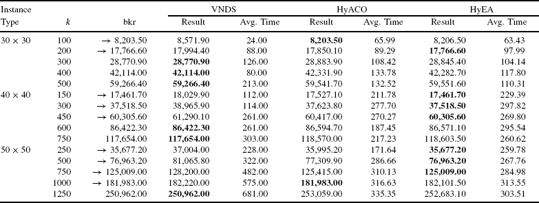
TABLE 23.4 Results for Edge-Weighted Random Graphs [29]

Acknowledgments

This work was supported by the Spanish MEC projects OPLINK (TIN2005-08818) and FORMALISM (TIN2007-66523), and by the Ramón y Cajal program of the Spanish Ministry of Science and Technology, of which Christian Blum is a research fellow.

REFERENCES

1. T. Bäck. Evolutionary Algorithms in Theory and Practice. Oxford University Press, New York, 1996.

2. C. Blum. A new hybrid evolutionary algorithm for the k-cardinality tree problem. In M. Keijzer et al., eds., Proceedings of the Genetic and Evolutionary Computation Conference 2006 (GECCO'06). ACM Press, New York, 2006, pp. 515–522.

3. C. Blum. Revisiting dynamic programming for finding optimal subtrees in trees. European Journal of Operational Research, 177(1):102–115, 2007.

4. C. Blum and M. Blesa. Combining ant colony optimization with dynamic programming for solving the k-cardinality tree problem. In Proceedings of the 8th International Work-Conference on Artificial Neural Networks, Computational Intelligence and Bioinspired Systems (IWANN'05), vol. 3512 of Lecture Notes in Computer Science. Springer-Verlag, New York, 2005, pp. 25–33.

5. C. Blum, M. Blesa, A. Roli, and M. Sampels, eds. Hybrid Metaheuristics: An Emergent Approach to Optimization, vol. 114 in Studies in Computational Intelligence. Springer-Verlag, New York, 2008.

6. C. Blum and M. J. Blesa. New metaheuristic approaches for the edge-weighted k-cardinality tree problem. Computers and Operations Research, 32(6):1355–1377, 2005.

7. C. Blum and M. Ehrgott. Local search algorithms for the k-cardinality tree problem. Discrete Applied Mathematics, 128:511–540, 2003.

8. R. Borndörfer, C. Ferreira, and A. Martin. Matrix decomposition by branch-and-cut. Technical report. Konrad-Zuse-Zentrum für Informationstechnik, Berlin, 1997.

9. R. Borndörfer, C. Ferreira, and A. Martin. Decomposing matrices into blocks. SIAM Journal on Optimization, 9(1):236–269, 1998.

10. J. Brimberg, D. , and N. . Variable neighborhood search for the vertex weighted k-cardinality tree problem. European Journal of Operational Research, 171(1):74–84, 2006.

11. T. N. Bui and G. Sundarraj. Ant system for the k-cardinality tree problem. In K. Deb et al., eds., Proceedings of the Genetic and Evolutionary Computation Conference (GECCO'2004), vol. 3102 of Lecture Notes in Computer Science. Springer-Verlag, New York, 2004, pp. 36–47.

12. S. Y. Cheung and A. Kumar. Efficient quorumcast routing algorithms. In Proceedings of INFOCOM'94. IEEE Press, Piscataway, NJ, 1994, pp. 840–847.

13. M. Dorigo. Optimization, learning and natural algorithms (in Italian). Ph.D. thesis, Dipartimento di Elettronica, Politecnico di Milano, Italy, 1992.

14. M. Dorigo, V. Maniezzo, and A. Colorni. Ant system: optimization by a colony of cooperating agents. IEEE Transactions on Systems, Man, and Cybernetics, Part B, 26(1):29–41, 1996.

15. M. Ehrgott and J. Freitag. K_TREE/K_SUBGRAPH: a program package for minimal weighted k-cardinality-trees and -subgraphs. European Journal of Operational Research, 1(93):214–225, 1996.

16. M. Ehrgott, J. Freitag, H. W. Hamacher, and F. Maffioli. Heuristics for the k-cardinality tree and subgraph problem. Asia-Pacific Journal of Operational Research, 14(1):87–114, 1997.

17. M. Fischetti, H. W. Hamacher, K. Jørnsten, and F. Maffioli. Weighted k-cardinality trees: complexity and polyhedral structure. Networks, 24:11–21, 1994.

18. L. R. Foulds and H. W. Hamacher. A new integer programming approach to (restricted) facilities layout problems allowing flexible facility shapes. Technical Report 1992-3. Department of Management Science, University of Waikato, New Zealand, 1992.

19. L. R. Foulds, H. W. Hamacher, and J. Wilson. Integer programming approaches to facilities layout models with forbidden areas. Annals of Operations Research, 81:405–417, 1998.

20. J. Freitag. Minimal k-cardinality trees (in German). Master's thesis, Department of Mathematics, University of Kaiserslautern, Germany, 1993.

21. N. Garg and D. Hochbaum. An O(log k) approximation algorithm for the k minimum spanning tree problem in the plane. Algorithmica, 18:111–121, 1997.

22. H. W. Hamacher and K. Joernsten. Optimal relinquishment according to the Norwegian petrol law: a combinatorial optimization approach. Technical Report 7/93. Norwegian School of Economics and Business Administration, Bergen, Norway, 1993.

23. H. W. Hamacher, K. Jörnsten, and F. Maffioli. Weighted k-cardinality trees. Technical Report 91.023. Dipartimento di Elettronica, Politecnico di Milano, Italy, 1991.

24. A. Hertz and D. Kobler. A framework for the description of evolutionary algorithms. European Journal of Operational Research, 126:1–12, 2000.

25. F. Maffioli. Finding a best subtree of a tree. Technical Report 91.041. Dipartimento di Elettronica, Politecnico di Milano, Italy, 1991.

26. M. V. Marathe, R. Ravi, S. S. Ravi, D. J. Rosenkrantz, and R. Sundaram. Spanning trees short or small. SIAM Journal on Discrete Mathematics, 9(2):178–200, 1996.

27. H. W. Philpott and N. Wormald. On the optimal extraction of ore from an open-cast mine. Technical Report. University of Auckland, New Zeland, 1997.

28. R. Uehara. The number of connected components in graphs and its applications. IEICE Technical Report COMP99-10. Natural Science Faculty, Komazawa University, Japan, 1999.

29. D. , J. Brimberg, and N. . Variable neighborhood decomposition search for the edge weighted k-cardinality tree problem. Computers and Operations Research, 31:1205–1213, 2004.