
I’m alive Oh oh, so alive I’m alive Oh oh, so alive ... My head is full of magic, baby And I can share this with you The feel I’m on top again, baby That’s got everything to do with you
—Love and Rockets, "So Alive"
The pièce de résistance of Mathematica 6 is its dynamic interactivity features. These features forced Wolfram to completely rethink and redesign its frontend. This had the unfortunate consequence of breaking many notebooks from version 5 and earlier, especially those that used graphics. However, it is my opinion that the gain was well worth the pain!
The interactive features of Mathematica 6 are even more impressive
when one considers that they sit on relatively few new functions. The
centerpiece of interactivity is the function Manipulate. Think of Manipulate as a very intelligent
user-interface generator. Manipulate’s power comes by virtue of its
ability to take any Mathematica expression plus a declarative
description of the expression’s variables and generate a mini embedded
GUI within the notebook for interacting with that expression. Of course,
there are always caveats, and an important feature of this chapter is to
help you get the best possible results with nontrivial Manipulate use cases.
The first five recipes of this chapter are intended to gradually
introduce the reader to Manipulate by
demonstrating increasingly sophisticated examples. These recipes are not
necessarily intended for direct use but rather to illustrate the basic
features and generality of Manipulate. Each recipe highlights a feature
of Manipulate or a subtlety
of its use in a particular context. Animate is a relative of Manipulate that puts its interactive features
in autonomous mode. 15.15 Animating an Expression focuses
on Animate and shows how animations
can be exported to Flash and other Web-friendly formats.
Many users will never need anything beyond Manipulate, but more advanced applications
require you to dig deeper and understand lower-level dynamic primitive
functions called Dynamic,
DynamicModule, and DynamicWrapper. 15.4 Creating Expressions for Which Value Dynamically
Updates shows how Dynamic is used in conjunction with Manipulate to achieve better performance or
smoother operation. DynamicModule is
a preferred alternative to Module
when working with dynamic content, and I use it liberally before
introducing it formally. The initial usage does not require you to know
more than its function as a scoping construct. 15.11 Improving Performance of Manipulate by Segregating Fast and
Slow Operations illustrates the
intimate relationship between Manipulate and DynamicModule and shows why you often want to
use DynamicModule directly. Many
useful dynamic techniques require the use of DynamicWrapper but, unfortunately (as of
version 7), this important function is undocumented in the help system.
15.8 Using Scratch Variables with DynamicModule to Balance Speed
Versus Space, 15.11 Improving Performance of Manipulate by Segregating Fast and
Slow Operations, and 15.16 Creating Custom Interfaces show some interesting use cases
for this hidden gem.
Note
You will get the most out of this chapter by downloading its associated notebook from the book’s website and playing along; see http://oreilly.com/catalog/9780596520991 .
You want to control the value of one or more variables via an interactive interface and see their values update as you interact with the interface.


This solution is strictly intended as a simple
introduction to Manipulate. As it
stands, it is not very practical because the variables are displayed
rather than used to compute. Still, there are some important
concepts.
The first concept is that Manipulate will automatically choose a
control type based on the structure of the constraints you place on a
variable’s value. The most common control is a slider. It is chosen
when a variable is specified with a minimum and maximum value. Out[3] below shows three variations of
this idea. The second example uses a specified increment, and the
third adds an initial value.

When a multiple-choice list is specified, you will get either a series of buttons or a drop-down list, depending on the number of choices.

When a variable is unconstrained or just specified with an
initial value, Manipulate infers an
edit control. In the first case, the variable begins with a null
value, so it is probably a good idea to provide an initial
value.

A second concept, illustrated in Out[6], is that a
single variable can be bound to multiple controls. This has the effect
of tying the controls together so a change in one control changes the
variable and is automatically reflected in the other controls bound to
that variable. It’s possible in this circumstance to violate the
constraints of one of the controls. In this case, Manipulate will display a red area in the
control that has the violated constraint.

A third concept is the ability to provide an arbitrary label by specifying the label after the initial value. The label can be any Mathematica expression.

This recipe is intended to illustrate that any Mathematica
expression that can be parametrized can be used with Manipulate.

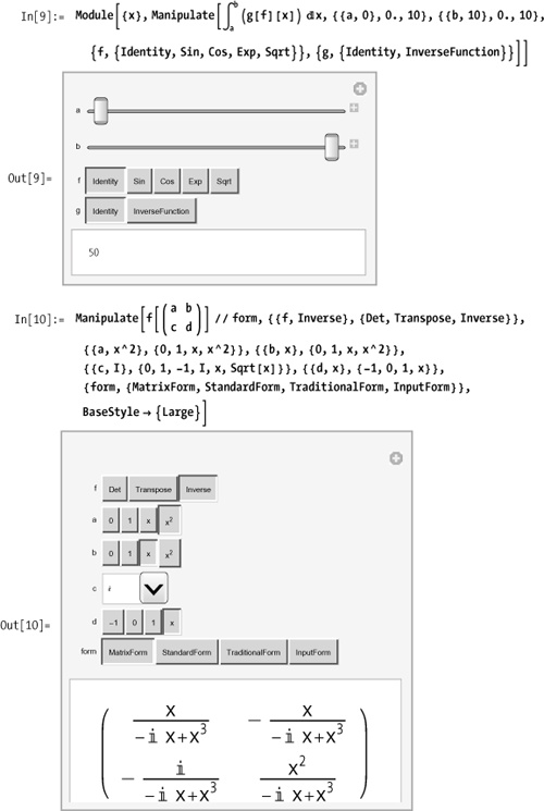
Here are a few examples to reinforce the idea that any aspect of
an expression can be manipulated. In Out[9] on Discussion, both of the function’s integration
limits are variable. In Out[10] on Discussion, every aspect of the expression,
including its display form, is subject to user manipulation. Finally,
in Out[11] on 15.3 Manipulating a Plot, you see that
tables of values can be dynamically generated and that Manipulate will adjust the display area to
accommodate the additional rows. The ability of Manipulate to mostly do the right thing is
immensely liberating: it allows you to focus on the concept you are
illustrating rather than the GUI programming.

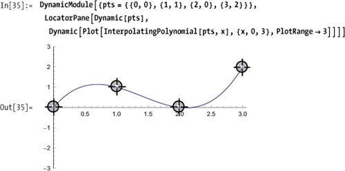
Possibly one of the most popular use cases for Manipulate is to create an interactive plot.
However, a common stumbling block is forgetting to specify the
PlotRange, causing a plot for which
the axes vary instead of the plot itself varying.

Use Mathematica to compare the solution to the following
variation and you will immediately see why PlotRange is essential.

Another common problem when manipulating graphics is
sluggishness when controls are varied. A crude way of dealing with
this problem is to tell Manipulate
to not update the display until the control is released. You do this
with the option ContinuousAction →
False.

A more refined alternative is to perform a low-resolution plot
while controls are changing and then switch automatically to a
full-resolution plot when the control is released. The ControlActive function along with PlotPoints is exactly what the doctor
ordered. Many graphics functions are self-adaptive when used inside a
Manipulate, but ControlActive allows you to fine-tune this
behavior to match the complexity of the graph and the speed of your
computer.

Another way to fine-tune interactive plots is to
separate those options that can be rendered quickly from those that
require a lot of computation. A classic example is a plot with
variable parameters that change the shape of the plot (expensive) and
parameters that change the orientation of the plot (inexpensive).
Ideally, parameters that are inexpensive to compute should not trigger
computation of the expensive parts. You achieve this by wrapping the
inexpensive parts in Dynamic[]. I
discuss this use of Dynamic in
detail in 15.11 Improving Performance of Manipulate by Segregating Fast and
Slow Operations.

You want to create output cells that have values that change in real time as variables used in computing the cell values change.
Normally an expression is evaluated and produces an output that
remains static. You can wrap an expression in Dynamic[] to indicate you want Mathematica
to update the value whenever a variable in the expression acquires a
new value. Here I initialize three variables and create a list in
which the first element is their sum and the second is the sum wrapped
in Dynamic. Initially the result is
{6,6} as you would expect. However,
you are looking at the output after the variable xl was given a new value of 100. Notice how the second element reflects
the new sum of 105.
In[17]:= xl = 1; x2 = 2; x3 = 3; {x1 + x2 + x3, Dynamic[x1 + x2 + x3]}
Out[17]= {6,105}

In[18]:= xl = 100
Out[18]= 100
Dynamic is one of the
low-level primitives that make the functionality of Manipulate possible. A typical use case of
Dynamic is creating free controls
that update a variable.
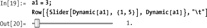
Dynamic expressions can appear in a variety of contexts and work
across multiple cells. Each output cell here will update as the slider
changes the value of a1.

There are two key principles that underlie Dynamic, and you must keep these in mind to
avoid common pitfalls. The first principle is that Dynamic has the attribute HoldFirst. This means that it does not
immediately update its expression until it needs to and does so only
to produce output.
In[24]:= Attributes[Dynamic]
Out[24]= {HoldFirst, Protected, ReadProtected}
This leads to the second key concept. Dynamic is strictly a frontend function and
can’t be used to produce values that will be passed to other
functions. The following example underscores this important
point.
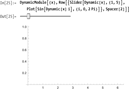
Moving the slider does nothing because passing the output of
Dynamic to a kernel function like
Sin can never work.
You want to apply a function to the output of a control
before it affects the value of a Dynamic expression.
Normally when you adjust a control, the value produced is
assigned to the expression in the first argument of Dynamic. However, if the expression is not a
variable that can be assigned, this will lead to errors. The solution
is provided by the second argument of Dynamic, which allows you to provide a
function that can override the default behavior. A classic example is
the creation of a control that inverts the value of the slider. Here
are a normal slider and an inverted slider that uses an inversion
function as its second argument.

The solution shows a case where the second argument of Dynamic is a function. Dynamic also supports a more advanced
variation where a list of functions is passed in the second argument.
A list with two functions tells Dynamic to evaluate the first function as
the control is varied and the second function when interaction with
the control is complete. A list with three functions defines a start
function, a during function, and an end function.

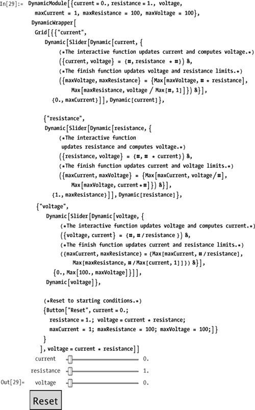
Here is an example illustrating Ohm’s law (voltage = current * resistance) as a set of three coupled sliders. The goal is for voltage to be computed when the current or resistance sliders change. However, if voltage is changed, then current must be recomputed. The problem with such an example is that if you allow voltage to change when resistance is high, it can easily lead to very large currents that would violate the limits of the current slider. The solution is to make the sliders’ limits dynamic as well, but that requires the whole slider to be dynamic! Of course, you don’t want the interface to be constantly generated as a slider is moved. This is where the finish function comes in handy. When a slider interaction ends, the limits of the other sliders are recomputed, triggering the creation of a new slider.
See 15.7 Using DynamicModule As a Scoping Construct in Interactive
Notebooks for an
explanation of why DynamicModule is
used in the Ohm’s law example.
You want to control the timing or variable dependencies that trigger and update to a dynamic value.
Use Refresh to explicitly
control dynamic updates. The following dynamic expression will
generate a random number once every second.

Also use Refresh to
control dependencies between dynamic variables. Here you create two
sliders that update the variables x
and y and two dynamic sums of
x and y, but you use Refresh to make the first sum respond to
changes in x alone, whereas the
second responds only to changes in y.

Refresh should be used with
caution because it subverts the expected behavior of Dynamic. One legitimate use of Refresh is with functions that will not be
triggered by Dynamic. Theodore Gray
of Wolfram Research refers to these functions as nonticklish. The
function Set normally written as
= is ticklish, as you can see by
evaluating the following expression.
In[33]:=  DynamicModule[{x = 1}, Dynamic[x = x + 1]]
Out[33]=  32872
This will create an output cell that increments about 20 times
per second, which is the standard refresh rate for Dynamic. Contrast this with the evaluation
of a nonticklish function, RandomReal.
In[34]:=  Dynamic[RandomReal[]]
Out[34]=  0.570894
This creates a single random number that will not update.
However, wrapping it with a Refresh, like we did in the Solution section above, will force it to
update.
You want to create dynamic content with local,
statically scoped variables (similar to Module) that maintain values across
sessions.
DynamicModule is similar to
Module in that it restricts the
scope of variables, but DynamicModule has the additional behavior of
preserving the values of the local variables in the output so that
they are retained between Mathematica sessions. Further, if you copy
and paste the output of a DynamicModule, the values of the pasted copy
are also localized in the copy, leaving the original unchanged as the
copy varies.
The dynamic plot on Discussion was copied from Out[35] above, pasted here, and then the locators manipulated. Each variable has its own independent state that will be retained after Mathematica is shut down and restarted with this notebook. This works because the values are bundled with the expression that underlies the output cells of a dynamic module.

Normal variables (including global variables and scoped
variables inside a Block or
Module) are stored inside the
Mathematica kernel’s memory. When the kernel exits, the values are
lost. DynamicModule variables are
stored in the notebook output cells. Below are a trivial DynamicModule and a trivial Module. Each simply sets a local variable to
1 and outputs the value. In Figure 15-1 and Figure 15-2 you can see the difference in
the underlying notebook representation (via ShowExpression).


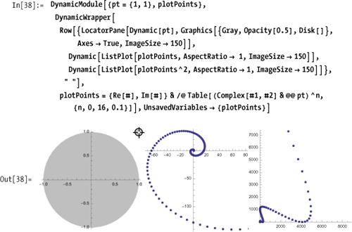
You want to avoid doing duplicate computations in a dynamic module by caching data, but you don’t want to create a bloated notebook when saved.
Use the UnsavedVariables
option of DynamicModule to prevent
saving in the notebook while keeping the variable localized in the
frontend. Also use DynamicWrapper
to guarantee cached data is calculated before any of the dynamic
expressions. In this example, you wish to compute plotPoints once since we plot the points and
their squares. You neither need nor want plotPoints to be saved in the notebook;
saving the locator point is sufficient.
My first attempt at the solution did not use DynamicWrapper and seemed to work fine.
However, as explained by Theodore Gray of Wolfram, there is a subtle
bug that will likely cause this to break in future versions of
Mathematica. The assumption is that the first Dynamic will be computed before the second,
and Mathematica provides no such evaluation order guarantee. In
contrast, the solution using DynamicWrapper will always guarantee that
the second argument of DynamicWrapper will be computed before any
dynamic expressions contained in the first argument.

DynamicWrapper is further
discussed in the DynamicWrapper: A Useful Undocumented Function sidebar on DynamicWrapper: A Useful Undocumented Function and the Discussion section of 15.11 Improving Performance of Manipulate by Segregating Fast and
Slow Operations.
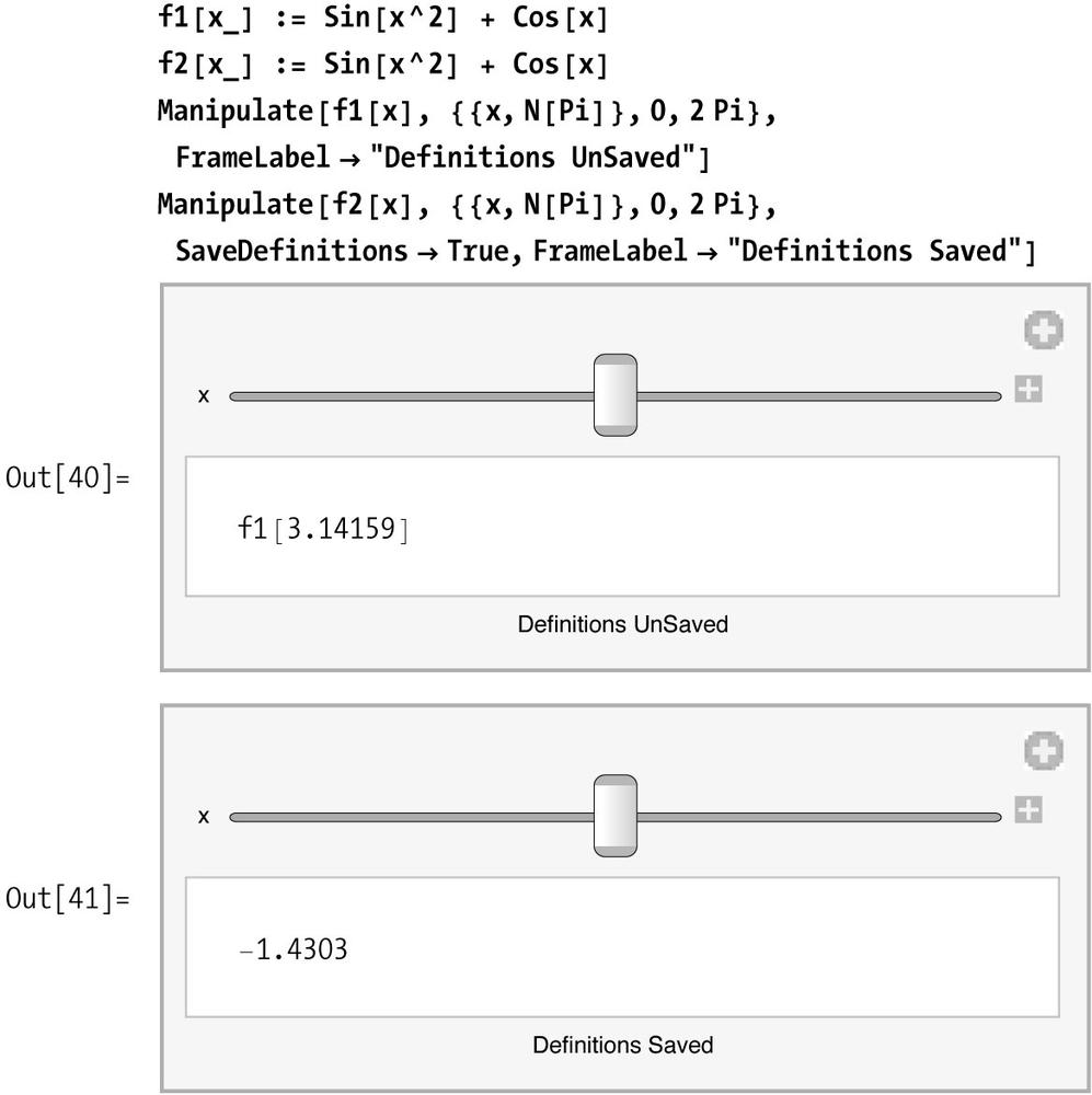
You want to make sure a Manipulate encapsulates all definitions
necessary for its operation so it always starts up in a working
state.
Manipulate can reference
functions and variables from the current kernel’s environment. There
is no guarantee that these will be defined or defined equivalently
when a notebook is saved and reopened. Compare the following two
cases. Although each Manipulate
below will behave the same after initial evaluation, you are seeing
the results after restarting Mathematica and reloading this notebook
without reevaluating the definitions of fl and f2. Note how the first does not know what
fl is, whereas the second remembers
the definition of f2 as
before.
For simple cases of self-contained formulas, the
solution using SaveDefinitions is
appropriate, but it has limitations. Although the definition of the
function is saved within the context of the manipulate output, it is
still in the Global` scope. This
means a Clear[f2] will break the
manipulation. To localize functions and variable definitions, you can
wrap the Manipulate in a DynamicModule. Now the variables defined in
the DynamicModule will be localized
and values will be preserved across Mathematica sessions.

Another potential problem with SaveDefinitions is that a great deal of code
can get pulled into the Manipulate
output. Imagine your Manipulate
uses a function that depends on code from an external package pulled
in by Needs. All the code in the
package could potentially be pulled into the Manipulate cell by SaveDefinitions. This will bloat the
notebook and affect the time it takes the control to initialize each
time. In situations like this, it is better to use the option Initialization. Further, if the Initialization code must complete before the
results are displayed, you should also specify option SynchronousInitialization → True.

You found some interesting results using Manipulate and want to preserve them for
future use.
Use the + icon in the Manipulate to select either "Paste Snapshot
" or "Add To Bookmarks."

In[46]:=  DynamicModule[{x = 4.8732500000000005`},
           -0.07` x5 - 0.42` x4 + 0.94` x3 - 4.25` x2 + 86.5` x - 0.13`]
Out[46]=   -0.00816536
You can bookmark specific settings by adjusting the dynamic module output to the desired values and then choosing "Add To Bookmarks." You will be prompted for a bookmark name. From that point on you can return to those settings by selecting the bookmark. In the figure below I have added two bookmarks: "Initial Settings" and "Interesting."

You have a sluggish Manipulate with several controls and you
would like to improve some aspects of its performance.
Isolate fast dynamic computations from computationally
intensive ones by performing the fast computations local to an
internal Dynamic. In the example
below, the generation of the 50,000 data points using NestList is significantly more expensive
than raising the values in the list to a power. You need not pay the
price of the generation when manipulating the variable z, but to isolate that computation you need
to wrap it in a Dynamic, as
shown.

This technique works because internally Manipulate wraps its expression with a
Dynamic and the net result is a
Dynamic nested inside another
Dynamic. In the solution, the inner
Dynamic is monitoring changes in
data and z but not r or x,
and since data does not recompute when z changes, data need not be recomputed. The
general rule is that changes that trigger only updates to an inner
Dynamic will not trigger updates to
any outer Dynamic.
You can also exploit this property when combining plots where
one is slow and the other is fast. To make this work, you need to
solicit the services of DynamicWrapper because Show cannot combine Dynamic output. The trick here is to use
DynamicWrapper to capture the
output of each plot, nesting the DynamicWrapper that computes the ReliefPlot (less expensive) inside the
DynamicWrapper that computes the
ListContourPlot (more expensive).
The result is that you can change the color function cf or the plot points p of the ReliefPlot and get fast updates while paying
for the updates to n or the number
of contours c only when these are
changed. The expression in In[50] was generated using
Maipulate’s Paste Sanpshot feature. Paste
Snapshot creates a static expression from the current
dynamic control settings.


Wrap the Manipulate in a DynamicModule and use the Initialization option to establish the
function’s definition. Below we define a global function f[x] and two Manipulates using localized definitions of
f[x] that remain
independent.
In[51]:= f[x_] := 1
Manipulate only localizes
variables associated with control variables. This can cause problems
when you have multiple Manipulates
that use the same function name in different ways. In Out[54] below,
it is clear that the second definition of g[x] modified the first since Sin[x] takes on values between -1 and
1.

Note that SaveDefinitions→
True as discussed in 15.9 Making a Manipulate Self-Contained does not localize the
symbol, so it is not a solution to this problem.

You want to create an interface that is divided across multiple cells or notebooks but interacts with shared variables. However, you don’t want these variables to be global.
Create a DynamicModule Wormhole using
InheritScope→ True from within a
Manipulate or DynamicModule you want to inherit
from.
Variables defined in the first argument of a DynamicModule or as control variables in a
Manipulate have their scope
restricted to the resulting output cell. This concept is explained in
15.7 Using DynamicModule As a Scoping Construct in Interactive
Notebooks.
Generally, this is exactly the behavior you want when using Manipulate. An obvious exception is when you
want to create a more complex application composed of multiple
notebooks (a palette is implemented as a notebook). The whimsical term
wormhole is used to suggest the sharing of scope
between different physical locations (e.g., output cells).
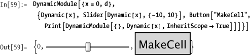
Here is an example that uses the same technique as the solution
but with DynamicModule instead of
Manipulate and multiple output
cells instead of a palette. Each time the button is pressed, a new
cell is printed that inherits the scope from the original DynamicModule.
The "Advanced Dynamic Functionality" tutorial
( http://bit.ly/3u8fXo )
explains some of the technical details underlying DynamicModule wormholes. It hints at the
ability to link up arbitrary existing DynamicModules but, unfortunately, provides
no additional information.
You want to create a control of your own design that can be used
inside a Manipulate or notebook
cell.
Manipulate allows you to
associate a control variable with a function and thus provides a means
to specify controls with nonstandard behavior and appearance. The
function incUntilButton creates a
button that increments the dynamic variable until it hits a specified
value, at which point it sets it back to the minimum specified in the
Manipulate definition. Notice how
the slider can change the x through
its full range while the button immediately resets x to -10 if it exceeds 5.

The function you use to create a custom control can take two
forms. In the simple form, it is passed only the control variable
wrapped in Dynamic (e.g., Dynamic[x]).

The solution shows the advanced form that gives the function
access to the minimum and maximum values specified in the definition.
In this case, the function Manipulate sees must have the form f[Dynamic[var_], {min_,max_}]. As the
solution shows, this does not mean you can’t use a function that takes
additional arguments. However, those arguments must be bound when the
anonymous function is created inside the Manipulate, as I did by providing "Inc Until 5" and 5 in the solution.
You may argue that a button hardly qualifies as a "custom
control" even though the solution gives it custom behavior. Have no
fear, because you have all the user interface primitives Mathematica
has to offer at your disposal for creating interesting controls. Here
is an example that shows how the angular slider (adapted from the
"Applications" section DynamicModule in the Mathematica
documentation) can be incorporated as a control in a Manipulate.

Use Animate to create
instructive self-running demonstrations. Here Animate drives an illustration of the
cycloid, which is the locus of points traced by a point on a wheel as
it rolls across a flat surface.

Animate can drive a
variety of demonstrations. Here we can get some insight into the
implementation of the Sort function
by providing a parameter limit
within a custom comparison function that short-circuits the sort after
that many steps. You use Animate
with BarChart to visualize the
partialSort at each step. Here the
option DisplayAllSteps keeps
Animate from skipping over steps.
DisplayAllSteps will slow things
down, so only use it if the animation suffers without it.

Other useful options are AnimationRunning→ True, which starts the
animation running immediately; AnimationRate, which sets the initial speed
of the animation; and AnimationRepetitions, which controls how
many times the animation repeats before stopping.
As you might expect, there is a close relationship
between Animate and Manipulate. Animate is implemented in terms of Manipulate with the help of a low-level
control called an Animator. You can
use an Animator directly to get
more control over the details of the animation layout. Stare at the
next animation for 10 seconds, and when you awaken, you will have the
strong urge to tell all your friends to buy the Mathematica
Cookbook!

You can share your animations over the Web by exporting them to
several common video formats, such as Microsoft AVI or Adobe Flash.
You may need to experiment with the options AnimationRate, RefreshRate, and DefaultDuration to get a smooth
animation.

The function ListAnimate provides an alternative to
Animate in which the animation is
derived by cycling through the elements of a list. This is useful in a
case where each step in the animation takes a lot of computation; you
can precompute all the frames of the animation and play them back
using ListAnimate. See the
Mathematica documentation for examples.
You want to create a custom interface that requires handling of low-level events such as mouse clicks.
Mathematica’s higher level interactive functionality is adequate
for most casual users, but sometimes you want to achieve something
cool. Luckily, Mathematica lets you intercept low-level GUI events
generated by your operating system using EventHandler. When you execute the following
code, you can increase the size of the text by dragging (moving the
mouse with the left button depressed) over the word Start. When you release the mouse, the text
changes to Done.

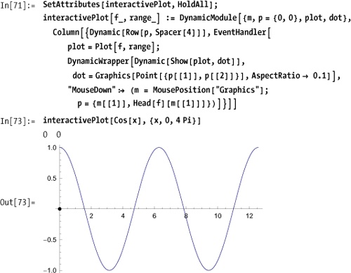
You can use event handlers to add interactive features to
existing plotting and graphics functions. In these applications, you
will often use MousePosition["Graphics"] to query the
position of the mouse relative to the enclosing graphic. Here interactivePlot creates a plot of a function
and annotates it with a point based on the position of the mouse when
you click. The coordinates of the point are displayed in the upper
left.
Event handlers can nest with the options PassEventsDown and PassEventsUp, controlling event propagation.
By default, inner event handlers get to act on events first, but outer
event handlers see the event first and thus can control propagation of
the event downward. The program below creates a simple game using the
keyboard. The idea is to try to catch the dot with the arrow. Notice
that there is an outer event handler that is used to control the
difficulty of the game using the d and e keys. The outer event handler
uses PassEventsDown → False, which means that if it handles the
event, then the inner handler will not see it. This prevents the dot
from moving when the d or e key is handled.

You want to go beyond what Manipulate has to offer and create your own
custom interfaces. You may need to manage a large number of controls
in a sensible manner or need a custom layout that Manipulate does not support.
The building blocks of sophisticated user interfaces are
PaneSelector and OpenerView, for managing many controls;
Control, for selection of
appropriate controls; and Item,
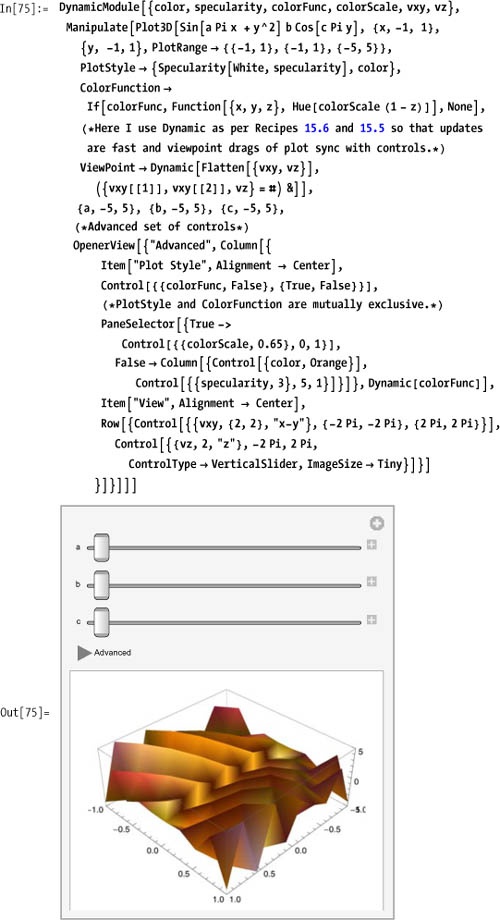
Row, Column, and Grid, for layout. The following Manipulate initially presents a simple
interface for modifying the parameters to a 3D plot. You use OpenerView to provide an advanced set of
controls that remain hidden until selected. Within this OpenerView, you use PaneSelector to alternate between sets of
controls, depending on a checkbox that allows modification of PlotStyle or ColorFunction.
In addition to OpenerView and PaneSelector, there is a whole family of
controls for managing limited screen real estate. These include
FlipView, MenuView, SlideView, and TabView. I provide a sample of each without
going into much detail because they are fairly self-explanatory and
follow the same basic syntax.
A FlipView cycles through a
list of expressions as you click on the output. Here I use FlipView over a list of graphics. Click on
the graphic to see the next in the series.

SlideView is similar to FlipView but uses VCR-style
controls to give more control of the progression.

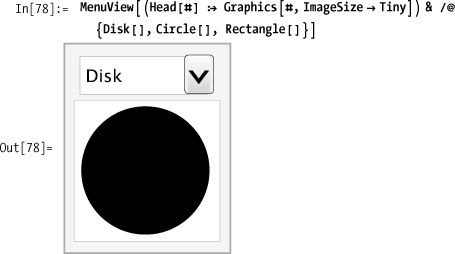
A MenuView allows you random
access to the items via a menu that you specify as a list of rules:
MenuView[{lbl1→expr1, label2→expr2,
        ...}]
. This is similar syntax to that used by PaneSelector in the solution. Don’t be
afraid to build up these expressions using a bit of functional
programming as I do here, especially if it cuts down on repetition. In
Out[78] below, I use the Head of
each graphic primitive as the label for convenience, but you can also
provide the label explicitly, as in Out[79] on Discussion, which builds the list of rules using Inner.

TabView is similar to
MenuView but uses the familiar
tabbed folder theme that has become popular in a variety of modern
interfaces, including most web browsers.

Clearly these controls can be mixed, combined with
Manipulate, or used alone to create
an unlimited variety of sophisticated interfaces. For example, here is
a tabbed set of Manipulates.

Contrast this to a single Manipulate that can switch between a
TabView or a MenuView, or even one that lets you switch
back and forth. This is actually a useful technique when building an
interface for someone’s approval. You can switch among various design
choices without touching the code.

Inspiration for this recipe came from a presentation by Lou D’Andria of Wolfram during the 2008 International Mathematica User Conference. Presentations from this conference can be found at http://bit.ly/41BMSZ .