You want to exploit your multicore computer by running two or more local kernels in parallel.

Use Edit, Preferences and navigate to the Parallel tab (see Figure 16-1). Within this top-level tab there is a subtab group where the first subtab is called Local Kernels. If you are configuring parallel preferences for the first time, this tab is probably already selected. Notice the button called Enable Local Kernels. Pressing that button will cause the display to change to that in Figure 16-2.

Figure 16-1. Parallel preferences for local kernel configuration

There are a few radio buttons for specifying how many slave kernels to run. The default setting is Automatic, meaning it will run as many kernels as there are cores, up to the standard license limit of four. For most users, this is exactly the setting you want, and you can now close the Preferences dialog and begin using the parallel programming primitives described in the remaining recipes of this chapter.

Figure 16-2. Preferences after enabling local kernels

The simplest way to get started with parallel computing in Mathematica is to run on a computer with more than one core. A four-core machine is ideal because that is the number of slave kernels Mathematica allows in a standard configuration. If you are using the computer to do other work, you may want to leave "Run kernels at lower process priority" checked, but on my Mac Pro eight-core processor, I uncheck this since there is plenty of CPU available to the system even with the four slaves, one master, and the frontend.

Once you have enabled local kernels, you can use Parallel Kernel Status to check the status of the slaves and launch or close them.

See 16.2 Configuring Remote Services Kernels for configuring access to kernels running on other computers on your network.

You want to exploit the computing resources of your network by running two or more kernels across multiple networked computers.

If you have not already done so, you must obtain the Lightweight Grid Service from Wolfram and install it on all computers that you wish to share kernels. The Lightweight Grid Service is available free to users who have Premier Service. Contact Wolfram for licensing details. By default, the Lightweight Grid Service is associated with port 3737, and assuming this default, you can administer the service remotely via a URL of the form http://<server name>:3737/WolframLightweightGrid/, where <server name> is replaced by the server or IP address. For example, I use http://maxwell.local:3737/WolframLightweightGrid/ for my Mac Pro. I could also access this machine via its IP address on my network http://10.0.1.4:3737/WolframLightweightGrid/.

Use the Lightweight Grid tab under Parallel Preferences tab to configure the Lightweight Grid. This tab should automatically detect machines on your local subnet. You can also find machines on other subnets (provided they are running Lightweight Grid) by using the "Discover More Kernels" option, and entering the name of the machine manually.

Figure 16-3. Parallel preferences for Lightweight Grid

Once you have the Lightweight Grid configured, remote kernels are as easy to use as local ones. Mathematica will launch the specified number of remote kernels on the computers you selected provided the kernels are available. The kernels may not be available if they are being used by another user on the network since each computer will typically have a maximum number of kernels that can be launched, and launching more kernels than there are cores on a specific computer does not usually make sense.

You can use the LaunchKernels command to launch kernels associated with a specific computer running the Lightweight Grid Service.

In[1]:= LaunchKernels["http://10.0.1.4:3737/WolframLightweightGrid/"];

Documentation and download links for the Lightweight Grid can be found at http://www.wolfram.com/products/lightweightgrid/.

You want to run a command on several kernels simultaneously.

Use ParallelEvaluate to send commands to multiple kernels and wait for results to complete. Use With to bind locally defined variables before distribution.

Imagine you need to generate many random numbers and you want to distribute the calculation across all available kernels. Here I use $KernelCount to make the computation independent of the number of kernels and Take to compensate for the extra numbers returned if $KernelCount does not divide 100 evenly.

In[2]:= Take[Flatten[ParallelEvaluate[
           RandomInteger[{-100, 100}, Ceiling[100/$KernelCount]]]], 100]
Out[2]= {83, -11, 5, -15, -11, -24, 6, -75, 74, 27, -42, 95, 100, -83, -91, -81, 25,
         -91, -96, -98, 9, 47, 44, 44, -81, 17, 10, -66, -40, -31, -30, 96, -55,
         92, -76, 5, -44, -79, -83, 51, -36, -93, -1, 12, 34, -68, -8, 29, 9, 1,
         44, 39, -1, 10, -80, -25, 62, 58, 88, -49, 77, 44, -48, 13, -69, -80, -39,
         -44, -37, 95, 34, -81, -8, 33, -79, 86, -97, 29, -29, -19, 22, 50, 4, 95,
         -55, -99, -98, 9, -61, -7, 0, -66, -14, -26, 95, 47, -35, -24, -29, -23}

In[3]:= Length[%]
Out[3]= 100

If you want to make the number of random numbers into a variable, you need to use With since variable values are not known across multiple kernels by default.

In[4]:= vars = With[{num =1000}, Take[Flatten[ParallelEvaluate[
               RandomInteger[{-100, 100}, Ceiling[num/$KernelCount]]]], num]];
         Length[
          vars]
Out[5]= 1000

Since ParallelEvaluate simply ships the command as stated to multiple kernels, there needs to be something that inherently makes the command different for each kernel; otherwise you just get the same result back multiple times.

You can control which kernels ParallelEvaluate uses by passing as a second argument the list of kernel objects you want to use. The available kernel objects are returned by the function Kernels[].

In[7]:= Kernels[]
Out[7]= {KernelObject[1, local], KernelObject[2, local],
         KernelObject [3, local], KernelObject [4, local]}

Here you evaluate the kernel ID and process ID of the first kernel returned by Kernels[] and then for all but the last kernel.

In[8]:=  link = Kernels[][[1]];
         ParallelEvaluate[{$KernelID, $ProcessID}, link]
Out[9]=  {1, 2478}

In[10]:= ParallelEvaluate[{$KernelID, $ProcessID}, Drop [Kernels [], 1]]
Out[10]= {{2, 2479}, {3, 2480}, {4, 2481}}

If you use Do or Table with ParallelEvaluate, you may not get the result you expect since the iterator variable will not be known on remote kernels. You must use With to bind the iteration variable before invoking ParallelEvaluate.

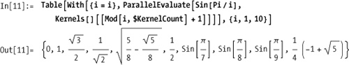
In any case, you don’t want to use ParallelEvaluate with Table because this will effectively serialize the computation across multiple kernels rather than execute them in parallel. You can see this by using AbsoluteTiming.

In[12]:= AbsoluteTiming[Table[ParallelEvaluate[Pause[1];
            0, Kernels[][[Mod[j, $KernelCount] + 1]]], {j, 1, 4}]]
Out[12]= {4.010592, {0, 0, 0, 0}}

ParallelEvaluate is useful for interrogating the remote kernels to check their state. For example, a common problem with parallel processing occurs when the remote kernels are not in sync with the master with respect to definitions of functions.

See the Mathematica documentation for ParallelTable and ParallelArray for better ways to parallelize Table-like operations.

You have code that you wrote previously in a serial fashion and you want to experiment with parallelization without rewriting.

Use Parallelize to have Mathematica decide how to distribute work across multiple kernels. To demonstrate, I first generate 1,000 large random semiprimes (composite numbers with only two factors).

In[16]:= semiprimes =
           Times @@@ Map[Prime, RandomInteger[{10000, 1000000}, {1000, 2}], {2}];
In[17]:= Prime[10000]
Out[17]= 104729

Using Parallelize, these semiprimes are factored in ~0.20 seconds.

In[18]:= {timing1, result} =
          AbsoluteTiming[Parallelize[Map[FactorInteger, semiprimes]]]; timing1
Out[18]= 0.206849

Running on a single kernel takes ~0.73 seconds, giving a 3.6 times speedup on my eight-core machine.

In[19]:= {timing2, result} = AbsoluteTiming[Map[FactorInteger, semiprimes]]; timing2
Out[19]= 0.737002
In[20]:= timing2/timing1
Out[20]= 3.563

If you replace AbsoluteTiming with Timing, you measure an 8 times speedup on this problem, so the cost of communicating results back to the frontend is significant.

In the solution, I did not use any user-defined functions, so Parallelize was all that was necessary. In a more realistic situation, you will first need to DistributeDefinitions of user-defined functions and constants to all kernels before using Parallelize.

In[21]:= fmaxFactor[x_Integer] := Max[Power @@@ FactorInteger[x]]
         fmaxFactor[1000]
Out[22]= 125

In[23]:= DistributeDefinitions[fmaxFactor];
         Parallelize[Map[fmaxFactor, semiprimes]] // Short
Out[24]= {11124193, 11988217, 12572531, 3331357, 15447821, 11540261,
          715643, 5844217, 9529441, 8574353, 3133597, 9773531, <<976>>,
          10027051, 7012807, 13236779, 13258519, 11375971, 7156727,
          13759661, 15155867, 13243157, 8888531, 11137717, 1340891}

Parallelize will consider listable functions, higher-order functions (e.g., Apply, Map, MapThread), reductions (e.g., Count, MemberQ), and iterations (Table).

There is a natural trade-off in parallelization between controlling the overhead of splitting a problem or keeping all cores busy. A coarse-grained approach splits the work into large chunks based on the number of kernels. If a kernel finishes its chunk first, it will remain idle as the other kernels complete their work. In contrast, a fine-grained approach uses smaller chunks and therefore has a better chance of keeping cores occupied, but the trade-off is increased communications overhead.

You can use Parallelize to implement a parallel version of MapIndexed since Mathematica 7 does not have this as a native operation (it does have ParallelMap, which I will discuss in 16.6 Implementing Data-Parallel Algorithms by Using ParallelMap).

You want to parallelize a function that can be fed chunks of a list in parallel and the intermediate results combined to yield the final answer.

Use ParallelCombine to automatically divvy up the processing among available kernels. Here we generate a list of integers and ask Mathematica to feed segments of the list to Total with each segment running on a different kernel. The individual totals are then combined with the function Plus to arrive at the grand total.

In[32]:= integersList = RandomInteger[{0, 10^8}, 10000000];
         ParallelCombine[Total, integersList, Plus]
Out[33]= 500 152 672 039 330

ParallelCombine can be applied to optimization problems where the goal is to find the best of a list of inputs. Here I use Max as the objective function, but in practice this would only be useful if the objective function was computationally intense enough to justify the parallel processing overhead. If the objective function is equally expensive for all inputs, you will want to specify Method—"CoarsestGrained".

To get actual speedup with ParallelCombine, you must pick problems for which the data returned from each kernel is much smaller than the data sent. Here is an example that has no hope for speedup even though on the surface it may seem compelling. Here, the idea is to speed up a Sort by using ParallelCombine to Sort smaller segments, and then perform a final merge on the sorted sections.

Here you can see that a plain Sort in a single kernel is an order of magnitude faster. If you think this has to do with using Sort[Flatten[#]] as the merge function, think again.

In[39]:= AbsoluteTiming[Sort[data ]] // Short
Out[39]= {0.018599, { 1, 1, 1, 1, 1, 1, 1, 1, 1, 1, 1, 1, 1, 1, 1, 1,
           1, 1, 1, 1, 1, 1, 1, 1, 1, 1, 1, 1, 1, <<99942>>, 100, 100, 100,
           100, 100, 100, 100, 100, 100, 100, 100, 100, 100, 100, 100, 100,
           100, 100, 100, 100, 100, 100, 100, 100, 100, 100, 100, 100, 100}}

Even if you use Identity to make the merge a no-op, the distributed "Sort" will be significantly slower. Adding more data or more process will not help because it only exacerbates the communications overhead.

You want to map a function across a list of data by executing the function in parallel for different items in a list.

Functional styles of programming often lead naturally to parallel implementation, especially when functions are side-effect free. ParallelMap is the parallel counterpart to Map (/@). It will spread the execution of the Map operation across available kernels.

In[41]:= ParallelMap[PrimeOmega, RandomInteger[{10^40, 10^50}, 32]]
Out[41]= {5, 5, 5, 5, 4, 2, 1, 6, 1, 7, 10, 7, 5, 7,
          6, 7, 7, 5, 4, 9, 10, 5, 7, 6, 4, 6, 8, 3, 12, 7, 7, 4}

Here I compare the performance of ParallelMap with regular Map on a machine running four slave kernels. You can see that the speedup is less than the theoretical limit due to overhead caused by communication with the kernels and other inefficiencies inherent in ParallelMap’s implementation.

ParallelMap is a natural way to introduce parallelism using a functional style. When you have a computationally intensive function you need to execute over a large data set, it often makes sense to execute the operations in parallel by allowing Mathematica to split the mapping among multiple kernels.

Like Map, ParallelMap can accept a levelspec as a third argument to control the parts of the expression that are mapped. For example, here I count the satisfiability count for all Boolean functions of one to four variables, where each function of a particular variable count is grouped together at level two in the list. The entire output is large, so I abbreviate using Short.

In[44]:= ParallelMap [SatisfiabilityCount [BooleanFunction@@#] &,
         Table[{n, v}, {v, 1,4}, {n, 1, 2^2^ v}], {2}] // Short
Out[44]= {{1, 1, 2, 0}, <<2>>, {1, 1, 2, 1, 2, 2, 3, 1, 2, 2, 3, 2, 3, 3, 4, 1, 2, 2, 3, 2,
           3, 3, 4, 2, 3, 3, 4, 3, 4, 4, 5, 1, 2, 2, 3, 2, 3, 3, <<65460>>, 14, 13,
           14, 14, 15, 11, 12, 12, 13, 12, 13, 13, 14, 12, 13, 13, 14, 13, 14, 14,
           15, 12, 13, 13, 14, 13, 14, 14, 15, 13, 14, 14, 15, 14, 15, 15, 16, 0}}

You have a problem that involves computation across a large data set, and you partition the data set into chunks that can be processed in parallel.

A simple example of this problem is where the computation occurs across a data set that can be generated by Table. Here you can simply substitute ParallelTable. For example, visualizing the Mandelbrot set requires performing an iterative computation on each point across a region of the complex plane and assigning a color based on how quickly the iteration explodes toward infinity. Here I use a simple grayscale mapping for simplicity.

ParallelTable has many useful applications. Plotting a large number of graphics is a perfect way to utilize a multicore computer. Parallel processing makes you a lot more productive when creating animations, for example.

You can also generate multiple data sets in parallel, which you can then plot or process further.

You want to parallelize an operation whose runtime varies greatly over different inputs.

The parallel primitives Parallelize, ParallelMap, ParallelTable, ParallelDo, ParallelSum, and ParallelCombine support an option called Method, which allows you to specify the granularity of subdivisions used to distribute the computation across kernels.

Use Method → "FinestGrained" when the completion time of each atomic unit of computation is expected to vary widely. "FinestGrained" prevents Mathematica from committing work units to a kernel until a scheduled work unit is complete. To illustrate this, create a function for which the completion time can be controlled via Pause. Then generate a list of small random delays and prepend to that a much larger delay to simulate a long-running computation.

In[50]:= SeedRandom[11];
         delays = RandomReal[{0.1, 0.15}, 200];
         (*Add a long
           20-second delay to simulate a bottleneck in the computation.*)
         PrependTo[delays, 20.0];
         funcWithDelay[delay_] := Module[{}, Pause[delay]; delay]
         DistributeDefinitions[funcWithDelay];

Since the pauses are distributed over several cores, we expect the actual delay to be less than the total delay, and that is what we get. However, by specifying "CoarsestGrained", we tell Mathematica to distribute large chunks of work to the kernels. This effectively results in jobs backing up behind the ~20-second delay.

When we run the same computation with Method → "FinestGrained", our actual completion time drops by 6 seconds since the remaining cores are free to receive more work units as soon as they complete a given work unit.

Contrast this to the case where the expected computation time is very uniform. Here Method → "CoarsestGrained" has a distinct advantage since there is less overhead in distributing work in one shot than incrementally.

Here we see that Method → "FinestGrained" only has a slight disadvantage, but that disadvantage would increase with larger payloads and remotely running kernels.

If you have ever been to the bank, chances are you stood in a single line that served several tellers. When a teller became free, the person at the head of the line went to that window. It turns out that this queuing organization produces higher overall throughput because different customers’ bank transactions take varying amounts of time, while presumably each teller is equally skilled at handling a variety of transactions. This setup is analogous to the effect you get when using "FinestGrained".

If there were no overhead involved in communication, "FinestGrained" would be ideal. But, returning to the analogy with the bank, it is often the case that the person who is next in line fails to notice a teller has become free and a delay is introduced. This is analogous to the master-slave overhead: the master must receive a result from the slave and move the next work unit into the freed-up slave. Each such action has overhead, and this overhead can swamp any gains obtained from making immediate use of an available slave.

In many problems, it is best to let Mathematica balance these trade-offs by using Method→Automatic, which is what you get by default when no Method is explicitly specified. Under this scenario, Mathematica performs a moderate amount of chunking of work units to minimize communication overhead while not committing too many units to a single slave and thus risking wasted computation when one slave finishes before the others.

There are a few less important Method options ("EvaluationsPerKernel" and "ItemsPerEvaluation") that are covered under the Parallelize function in Mathematica’s documentation. These give you more precise control over the distribution of work.

You have several different ways to solve a problem and are uncertain which will complete fastest. Typically, one algorithm may be faster on some inputs, while another will be faster on other inputs. There is no simple computation that makes this determination at lower cost than running the algorithms themselves.

Use ParallelTry to run as many versions of your algorithm as you have available slave kernels. There are several ways to use ParallelTry, but the differences are largely syntactical. If your algorithms are implemented in separate functions (e.g., algo1[data_], algo2[data_], and algo3[data_]), you can use ParallelTry, as in the following example. Here I merely simulate the uncertainty of first completion using a random pause.

In[57]:= RandomSeed[13];
         algo1[data_] := Module[{}, Pause[RandomInteger[{1, 10}]]; data^2]
         algo2[data_] := Module[{}, Pause[RandomInteger[{1, 10}]]; data^3]
         algo3[data_] := Module[{}, Pause[RandomInteger[{1, 10}]]; data^4]
         DistributeDefinitions[algo1, algo2, algo3]
         algo[data_] := ParallelTry[Composition[#][data] &, {algo1, algo2, algo3}]
In[59]:= algo[2]
Out[59]= 4

Sometimes you can choose variations to try by passing different function arguments. Here I minimize a BooleanFunction of 30 variables using ParallelTry with four of the forms supported by BooleanMinimize.

In[60]:= ParallelTry[{#, BooleanMinimize[BooleanFunction[10000, 30], #]} &,
          {"DNF", "CNF", "NAND", "NOR"}]
Out[60]= {CNF, ! #1 && ! #2 && ! #3 && ! #4 && ! #5 && ! #6 && ! #7 && ! #8 &&
             ! #9 && ! #10 && ! #11 && ! #12 && ! #13 && ! #14 && ! #15 && ! #16 &&
             ! #17 && ! #18 && ! #19 && ! #20 && ! #21 && ! #22 && ! #23 && ! # 24 &&
             ! #25 && ! #26 && (! #27 || ! #28 || #30) &&(#27 || #28) &&
             (#27 || ! #30) &&(! #28 || ! #29) &&(! #29 || ! #30) &}

Another possibility is that you have a single function that takes different options, indicating different computational methods. Many advanced numerical algorithms in Mathematica are packaged in this manner.

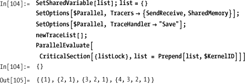
Your parallel implementations need to communicate via one or more variables shared across kernels.

Mathematica provides SetSharedVariable as a means of declaring one or more variables as synchronized across all parallel kernels. Similarly, SetSharedFunction is used to synchronize the down values of a symbol. In the following example, the variable list is shared and each slave kernel is thus able to prepend its $KernelID.

In[64]:= SetSharedVariable[list]; list = {};
         ParallelEvaluate[PrependTo[list, $KernelID]];
         list
Out[65]= {4,3,2,1}

Consider a combinatorial optimization problem like the traveling salesperson problem (TSP). You might want all kernels to be aware of the best solution found by any given kernel thus far so that each kernel can use this information to avoid pursuing suboptimal solutions. Here I use a solution to the TSP based on simulated annealing.

In[66]:= dist = Table[lf[i <= j, 0, RandomReal [{1, 10}]], {i, 1, 10}, {j, 1, i}];

Prior to Mathematica 7, users never had to think about problems like race conditions because all processing occurred in a single thread of execution. Parallel processing creates the possibility of subtle bugs caused by two or more kernels accessing a shared resource such as the file system or variables that are shared. These resources are not subject to atomic update or synchronization unless special care is taken.

Consider a situation where each parallel task needs to update a shared data structure like a list. Here I create a simplified example with a shared list. Each kernel is instructed to prepend its $KernelID to the list 10 times. If all goes well, we should see 10 IDs for each kernel. I use Tally to see if that is the case. The random pause is there to inject a bit of unpredictability into each computation to simulate a more realistic computation.

In[67]:= SetSharedVariable[aList]; aList = {};
         ParallelEvaluate[Do[aList = Prepend [aList, $KernelID];
            Pause[ RandomReal[{ 0.01, 0.1}]], { 10}]];
         Tally[
          aList]
Out[68]= {{2, 7}, {1, 8}, {3, 4}, {4, 7}}

Clearly this is not the result expected, since not one of the $KernelID's showed up 10 times. The problem is that each kernel may interfere with the others as it attempts to modify the shared list. This problem is solved by the use of CriticalSection.

In[69]:= SetSharedVariable[aList]; aList = {};
         ParallelEvaluate[
           Do[CriticalSection[{aListLock}, aList = Prepend [aList, $KernelID]];
            Pause[ RandomReal[{0.01, 0.1}]], {10}]];
         Tally[
          aList]
Out[70]= {{4, 10}, {3, 10}, {1, 10}, {2, 10}}

Much better. Now each kernel ID appears exactly 10 times.

A critical section is a mutual exclusion primitive implemented in terms of one or more locks. The variables passed, as in the list (first argument to CriticalSection), play the role of the locks. A kernel must get control of all locks before it is allowed to enter the critical section. You may wonder why you would ever need more than one lock variable. Consider the case where there are two shared resources and three functions that may be executing in parallel. Function f1 accesses resource r1, which is protected by lock 11. Function f2 accesses resource r2, which is protected by lock 12. However, function f3 accesses both r1 and r2, so it must establish both locks. The following example illustrates.

In[71]:= SetSharedVariable[r1, r2, r3];
         r1 = {}; r2 = {}; r3 = {};
         f1[x_] :=
          Module[{}, CriticalSection[{11}, PrependTo[r1, x]]]
         f2[x_] :=
          Module [{}, CriticalSection [{12}, PrependTo[r2, x ]]]
         f3[] :=
          Module[{}, CriticalSection[{11, 12}, r3 = Join[r1, r2]]]

If f1, f2, and f3 happen to be running in three different kernels, f1 and f2 will be able to enter their critical sections simultaneously because they depend on different locks, but f3 will be excluded. Likewise, if f3 has managed to enter its critical section, both f1 and f2 will be locked out until f3 exits its critical section.

Keep in mind that shared resources are not only variables used with SetShared-Variable. They might be any resource that a kernel could gain simultaneous access to, including the computer’s file system, a database, and so on.

It should not come as a surprise that critical sections can reduce parallel processing performance since they effectively define sections of code that can only execute in one kernel at a time. Further, there is a loss of liveliness since a kernel that is waiting on a lock cannot detect instantaneously that the lock has been freed. In fact, if you dig into the implementation (the entire source code for Mathematica 7’s parallel processing primitives is available in Parallel.m and Concurrency.m) you will see that a kernel enters into a 0.1-second pause while waiting on a lock. This implies that CriticalSection should be used sparingly, and if possible, you should find ways to structure a program to avoid it altogether. One obvious way to do this is to rely largely on the data parallelism primitives like ParallelMap and ParallelTable and only integrate results of these operations in the master kernel. However, advanced users may want to experiment with more subtle parallel program designs, and it is handy that synchronization is available right out of the box.

In 16.13 Processing a Massive Number of Files Using the Map-Reduce Technique, I implement the map-reduce algorithm where CriticalSection is necessary to synchronize access to the file system.

You have a computation that involves processing many data sets where the computation can be viewed as data flowing through several processing steps. This type of computation is analogous to an assembly line.

An easy way to organize a pipeline is to create a kind of to-do list and associate it with each data set. The master kernel loads the data, tacks on the to-do list and a job identifier, and then submits the computations to an available slave kernel using ParallelSubmit. The slave takes the first operation off the to-do list, performs the operation, and returns the result to the master along with the to-do list and job identifier it was given. The master then records the operation as complete by removing the first item in the to-do list and submits the data again for the next step. Processing is complete when the to-do list is empty. Here I use Reap and Sow to collect the final results.

In[73]:= slaveHandler[input_, todo_,jobId_] := Module[{result},
           result = First [todo][input];
           {todo, result, jobId}
          ]

          DistributeDefinitions[slaveHandler];

          pipelineProcessor[ inputs_, todo_] :=
           Module[{ pids, result, id},
            Reap[
             pids = With[{todo1 = todo},
               MapIndexed[ParallelSubmit[slaveHandler[#, todo1,
                   First[#2]]] &, inputs]];
             While[pids =!= {},
              {result, id, pids} = WaitNext[pids];
              If[Length[result[[1]]] > 1,
               AppendTo[pids,
                With[{todo1 = Rest[result[[1]]], in = result[[2]], jobId =
                   result[[3]]}, ParallelSubmit[slaveHandler[in, todo1, jobId]]]],
               Sow[{Last[FileNameSplit[inputs[[result[[3]]]]]], result[[2]]}
                ];

              ]
             ];
             True
            ]
           ]

To illustrate this technique, I use an image-processing problem. In this problem, a number of images need to be loaded, resized, sharpened, and then rotated. For simplicity, I assume all images will use the same parameters. You can see that the to-do list is manifested as a list of functions.

The solution illustrates a few points about using ParallelSubmit that are worth noting even if you have no immediate need to use a pipeline approach to parallelism.

First, note the use of MapIndexed as the initial launching pad for the jobs. MapIndexed is ideal for this purpose because the generated index is perfect as a job identifier. The jobId plays no role in slaveHandler but is simply returned back to the master. This jobId allows the master to know what initial inputs were sent to the responding slave. Similarly, you may wonder why the whole to-do list is sent to the slave if it is only going to process the first entry. The motivation is simple. This approach frees pipelineProcessor from state management. Every time it receives a response from a slave, it knows immediately what functions are left for that particular job. This approach is sometimes called stateless because neither the master nor the slaves need to maintain state past the point where one transfers control to the other.

Also note the use of With as a means of evaluating expressions before they appear inside the arguments of ParallelSubmit. This is important because ParallelSubmit keeps expressions in held form and evaluating those expressions on slave cores is likely to fail because the data symbols (like todo and result) don’t exist there.

A reasonable question to ask is, why use this approach at all? For instance, if you know you want to perform five operations on an image in sequence, why not just wrap them up in a function and use ParallelMap to distribute images for processing? For some cases, this approach is indeed appropriate. There are a few reasons why a pipeline technique might still make sense.

Intermediate results

Checkpointing

Managing complexity

Branching pipelines

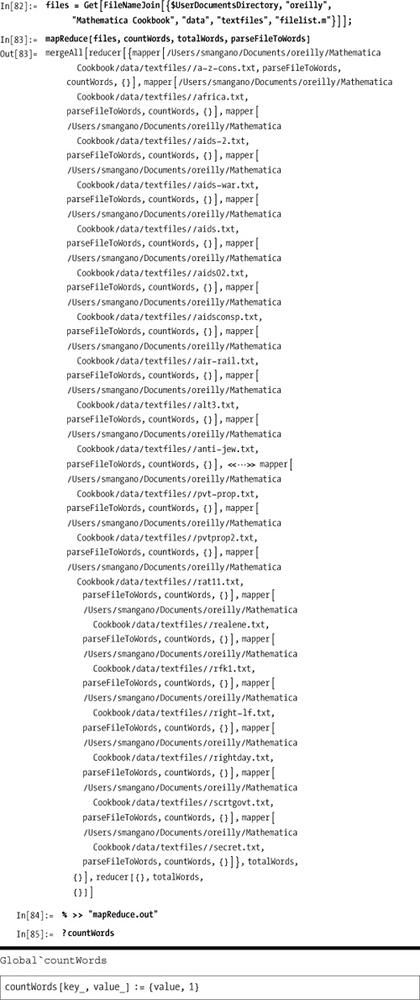
You have a large number of data files that you need to process. Typically you need to integrate information from these files into some global statistics or create an index, sort, or cross-reference. The data from these files is too large to load into a single Mathematica kernel.

Here I show a toy use case traditionally used to introduce mapReduce. The problem is to process a large number of text files and calculate word frequencies. The principle that makes mapReduce so attractive is that the user need only specify two, often simple, functions called the map function and the reduce function. The framework does the rest. The map function takes a key and a value and outputs a different key and a different value. The reduce function takes the key that was output by map and the list of all values that map assigned to the specific key. The framework’s job is to distribute the work of the map and reduce functions across a large number of processors on a network and to group by key the data output by map before passing it to reduce.

To make this concrete, I show how to implement the word-counting problem and the top-level mapReduce infrastructure. In the discussion, I dive deeper into the nuts and bolts.

First we need a map function. Recall that it takes a key and a value. Let’s say the key is the name of a file and the value is a word that has been extracted from that file. The output of the map function is another key and value. What should these outputs be to implement word counting? The simplest possible answer is that the output key should be the word and the output value is simply 1, indicating the word has been counted. Note that the input key (the filename) is discarded, which is perfectly legitimate if you have no need for it. In this case, I do not wish to track the word’s source.

In[77]:= countWords[key_, value_] := {value, 1}

Okay, that was easy. Now we need a reduce function. Recall that the reduce function will receive a key and a list of all values associated to the key by the map function. For the case at hand, it means reduce will receive a word and a list of 1’s representing each time that word was seen. Since the goal is to count words, the reduce function simply performs a total on the list. What could be easier?

In[78]:= totalWords[key_, value_List] := Total[value]

Here again I discard the key because the framework will automatically associate the key to the output of reduce. In other applications, the key might be required for the computation.

Surprisingly enough, these two functions largely complete the solution to the problem! Of course, something is missing, namely the map-reduce implementation that glues everything together. Here is the top-level function that does the work.

You can see from this function that it requires a list of inputs. That will be the list of files to process. It needs a function map, which in this example will be count-Words, and a function reduce, which will be totalWords. It also needs something called a parser. The parser is a function that breaks up the input file into the units that map will process. Here I use a simple parser that breaks up a file into words. This function leverages Mathematica’s I/O primitive ReadList, which does most of the work. The only bit of postprocessing is to strip some common punctuation that Read-List does not strip and to convert words to lowercase so counting is case insensitive.

In[81]:= parseFileToWords[file_] := Module[{stream, words},
           stream = OpenRead[file];
           words = ToLowerCase[Select[ReadList[stream, Word], StringMatchQ[#,
                RegularExpression["^[A-Za-z0-9][A-Za-z0-9-]*$"]] &]];
           Close[stream];
           words
          ]

Here is how you use the framework in practice. For test data, I downloaded a bunch of files from http://www.textfiles.com/conspiracy/. I placed the names of these files in another file called wordcountfiles and use Get to input this list. This is to avoid cluttering the solution with all these files.

If you want to try map-reduce, use the package files Dictionary.m and MapReduce.m. The code here is laid out primarily for explanation purposes. You will need to add the following code to your notebook, and don’t forget to use DistributeDefinitions with the functions you create for map, reduce, and parse.

Needs["Cookbook'Dictionary'"]
Needs["Cookbook'MapReduce'"]
ParallelNeeds["Cookbook'Dictionary'"]
ParallelNeeds["Cookbook~MapReduce~"]

You can find examples of usage in mapReduce.nb.

If you are new to map-reduce you should refer to references listed in the See Also section before trying to wrap your mind around the low-level implementation. The original paper by the Google researchers provides the fastest high-level overview and lists additional applications beyond the word-counting problem. The most important point about map-reduce is that it is not an efficient way to use parallel processing unless you have a very large number of files to process and a very large number of networked CPUs to work on the processing. The ideal use case is a problem for which the data is far too large to fit in the memory of a single computer, mandating that the processing be spread across many machines. To illustrate, consider how you might implement word counting across a small number of files.

The guts of our map-reduce implementation are a bit more complex than the other parallel recipes. The low-level implementation details have less to do with parallel processing than with managing the data as it flows though the distributed algorithm. A key data structure used is a dictionary which stores the intermediate results of a single file in memory. This makes use of a packaged version of code I introduced in 3.13 Exploiting Mathematica’s Built-In Associative Lookup and won’t repeat here.

The function mapAndStore is responsible for applying the map function to a key value pair and storing the result in a dictionary. The dictionary solves the problem of grouping all identical keys for a given input file.

In[88]:= mapAndStore[{key1_, value1_}, map_, dict_Dictionary] :=
          Module[{key2, value2},
           {key2, value2} = map[keyl, valuel];
           If[key2 =!= Null,
            dictStore[dict, key2, value2]]
          ]

The default behavior of mapReduce is to store intermediate results in a file. The functions uniqueFileName, nextUniqueFile, and saver have the responsibility of synthesizing the names of these files and storing the results. The filename is derived from the key, and options saveDirectory and keyToFilenamePrefix help to customize the behavior. These options are provided in the top-level mapReduce call. Here save-Directory provides a directory where the intermediate files will be stored. This directory must be writable by all slave kernels. Use keyToFilenamePrefix to specify a function that maps the key to a filename prefix. This function is necessary for cases where the key might not represent a valid filename.

The function mapper provides the glue between the parser, the map function, and the intermediate storage of the output of map. As mentioned above, the default behavior is to store the output in a file whose name is derived from the key. However, for small toy problems you might wish to dispense with the intermediate storage and return the actual output to the next stage of processing in the master kernel. This feature is available by specifying intermediateFile → False (the default is True).

Before the results of mapper can be passed to the reduce stage of processing, it is necessary to group all intermediate results together. For example, in the solution, we presented the problem of counting words in files. Consider a common word like the. Clearly, this word will have been found in almost all of the files. Thus, counts of this word are distributed across a bunch of intermediate files (or lists if intermediate-File→False was specified). Before the final reduction, the intermediate files (or lists) must be grouped by key and merged. This is the job of the functions mergeAll and merge. The grouping task is solved by the Mathematica 7 function GatherBy, and the actual merging is implemented as a parallel operation since each key can be processed independently.

The final stage is the reducer, which accepts the merged results (in file or list form) for each key and passes the key and resulting list to the reduce function. An option, fileDisposition, is used to determine what should happen to the intermediate file. The default disposition is DeleteFile, but you could imagine adding some more complex processing at this stage, such as logging or checkpointing a transaction that began during the parsing stage.

The original paper on map-reduce can be found at http://bit.ly/cqBSTH.

More details that were left out of the original paper can be found in the analysis at http://bit.ly/bXsWsD.

You are trying to understand why your parallel program is not achieving the expected speedup.

You can enable parallel tracing by setting options associated with the symbol $Parallel. Use Tracers to specify the types of trace information you want to output and TraceHandler to specify how the trace information should be processed.

Be sure to disable tracing when you are done.

There are four kinds of Tracers, and you can enable any combination of these. Each focuses on a different aspect of Mathematica’s parallel architecture.

In[99]:= OptionValues[Tracers]
Out[99]= {MathLink, Queueing, SendReceive, SharedMemory}

In addition, there are three ways to present the data via the TraceHandler option. Print and Display are similar, but Save is interesting because it defers output until the TraceList[] command is invoked.

Now when you execute TraceList, it will return the trace information in a list instead of printing it. This is useful if you want to further process this data in some way.

In[103]:= TraceList []
Out[103]= {{SendReceive,
           Sending to kernel 4: iid8608 [Table [Prime [i], {i, 99990, 99992, 1}]]
             (q=0)}, {SendReceive, Sending to kernel 3:
             iid8609 [Table[Prime[i], {i, 99993, 99995, 1}]](q=0)}, {SendReceive,
           Sending to kernel 2: iid8610 [Table [Prime [i], {i, 99996, 99998, 1}]]
             (q=0)}, {SendReceive,
           Sending to kernel 1: iid8611[Table[Prime[i], {i, 99999, 100001, 1}]]
             (q=0)}, {SendReceive,
           Receiving from kernel 4: iid8608 [{1299541, 1299553, 1299583}](q=0)},
          {Queueing, eid8608[Table[Prime[i], {i, 99990, 99992, 1}]] done},
          {SendReceive,
           Sending to kernel 4: iid8612[Table[Prime[i], {i, 100002, 100004, 1}]]
             (q=0)},  {SendReceive,
           Receiving from kernel 3: iid8609[{1299601, 1299631, 1299637}] (q=0)},
          {Queueing, eid8609[Table[Prime[i], {i, 99993, 99995, 1}]] done},
          {SendReceive,
           Sending to kernel 3: iid8613[Table[Prime[i], {i, 100005, 100006, 1}]]
             (q=0)}, {SendReceive,
           Receiving from kernel 2: iid8610[{1299647, 1299653, 1299673}] (q=0)},
          {Queueing, eid8610[Table[Prime[i], {i, 99996, 99998, 1}]] done},
          {SendReceive,
           Sending to kernel 2: iid8614[Table[Prime[i], {i, 100007, 100008, 1}]]
             (q=0)}, {SendReceive,
           Receiving from kernel 1: iid8611[{1299689, 1299709, 1299721}] (q=0)},
          {Queueing, eid8611[Table[Prime[i], {i, 99999, 100001, 1}]] done},
          {SendReceive,
           Sending to kernel 1: iid8615[Table[Prime[i], {i, 100009, 100010, 1}]]
             (q=0)}, {SendReceive,
           Receiving from kernel 4: iid8612[{1299743, 1299763, 1299791}] (q=0)},
          {Queueing, eid8612[Table[Prime[i], {i, 100002, 100004, 1}]] done},
          {SendReceive, Receiving from kernel 3: iid8613[{1299811, 1299817}] (q=0)},
          {Queueing, eid8613[Table[Prime[i], {i, 100005, 100006, 1}]] done},
          {SendReceive, Receiving from kernel 2: iid8614[{1299821, 1299827}] (q=0)},
          {Queueing, eid8614[Table[Prime[i], {i, 100007, 100008, 1}]] done},
          {SendReceive, Receiving from kernel 1: iid8615[{1299833, 1299841}] (q=0)},
          {Queueing, eid8615[Table[Prime[i], {i, 100009, 100010, 1}]] done}}

You can get a better understanding of the use of shared memory and critical sections by using the SharedMemory tracer.

Now executing TraceList shows how a shared variable was accessed and modified over the parallel evaluation as well as how locks were set and released.

It is enlightening to do the same trace without the use of CriticalSection. Here you can see the problems caused by unsynchronized modification of shared memory.

You want to get a handle on the inherent data communications overhead of parallel Mathematica in your environment.

Given that Mathematica is available on many operating systems and classes of computer, and also given that computational cores may be local or networked, and given network topologies and throughput, it is important to benchmark your environment to get a sense of its parallel performance characteristics.

One solution is to plot the time it takes to send various amounts of data to kernels with and without computation taking place on the data. The code below generates random data of various sizes and measures the time it takes to execute a function on that data on all kernels using ParallelEvaluate. Here I plot the Identity versus Sqrt versus Total to show the effect of no computation versus computation on every element of data versus computation on every element with a single return value. The key here is that the amount of data sent to slaves and returned to master is the same in the first two cases, whereas for the third case (dotted), less data is returned than sent. Also, the first case (solid) does no computation, and the second (dashed) and third (dotted) do.

The plot shows that communication overhead of sending data to kernels dominates since the effect of computing Sqrt is negligible. Also, Total (dotted) performs better because less data is returned to the master. Notice how the overhead is roughly linear within my configuration, which consists of four local cores on a Mac Pro with 4 GB of memory.

Many users who experiment casually with parallelization in Mathematica 7 come away disappointed. This is unfortunate because there are quite a few useful problems where parallel primitives can yield real gains. The trick is to understand the inherent overhead of your computational setup. Running simple experiments like the one in the solution can give you a sense of the limitations. There are many calculations Mathematica can do that take well under 0.05 seconds, but that is how long it might take to get your data shipped to another kernel. This can make parallelization impractical for your problem.

Consider the Mandelbrot plot from 16.7 Decomposing a Problem into Parallel Data Sets. Why did I achieve speedup there? The key characteristics of that problem are that very little data is shipped to the kernels, much computation is done with the data sent, and no coordination is needed with kernels solving other parts of the problem. Such problems are called embarrassingly parallel because it is virtually guaranteed that you will get almost linear speedup with the number of cores at your disposal.

Unfortunately, many problems you come across are not embarrassingly parallel, and you will have to work hard to exploit any parallelism that exists. In many cases, if you can achieve any speedup at all, you will need to expend much effort in reorganizing the problem to fit the computational resources you have at your disposal. The keys to success are: