
CHAPTER 13
PLANAR GRAPHS, GEOBOARDS, AND BRUSSELS SPROUTS
In the previous chapter we saw Cauchy’s clever technique for proving Euler’s formula. He took a polyhedron, removed a face, and projected the rest down onto the plane. Then he proved that V − E + F = 1 for this figure, so V − E + F = 2 for the polyhedron. The connection to graph theory should be obvious. At first glance it appears that it would be trivial to generalize Euler’s formula to graphs that are not projections of polyhedra and which may possess edges that are curved.
The difficulty with extending Euler’s formula is that it does not apply to every graph. Counting vertices and edges is easy—they are the building blocks from which graphs are made—but a graph need not have faces. Even when a graph is drawn on paper, the edges may not divide the region into faces. For example, the edge PR in the left-hand graph of figure 13.1 crosses edge QS, so it cannot be the boundary of a face. However, the graph can be redrawn (as on the right) without any crossings, thus dividing the region into faces. A graph that can be drawn without edges crossing is called planar.
On a polyhedron, a face is a region bounded by a polygon. For graphs, we adopt a looser definition. A face can be bounded by one edge, like the loop from P to P in figure 13.1. A face can be bounded by two edges, such as the pair of edges from Q to R. (A pair of edges that connect the same two vertices is called parallel.) A face may even have an edge protruding into its interior, such as the edge from S to T.

Figure 13.1. Two representations of the same graph.

Figure 13.2. Placing a planar graph on a sphere.
Many graph theorists count the exterior region as a face. If the graph is viewed as an island, then this unbounded face is the sea stretching off to infinity in every direction. Although it is somewhat inelegant to call this unbounded region a face, it is often more useful to include it than to exclude it. One way to reconcile this problem is to envision the graph as an island not on an unending sea, but on a globe (figure 13.2). In this way the unbounded face becomes finite.
So we have the following generalization of Euler’s formula for planar graphs.
EULER’S FORMULA FOR PLANAR GRAPHS
A connected planar graph with V vertices, E edges, and F faces satisfies V − E + F = 2.
If we do not count the unbounded region as a face, then Euler’s formula is V − E + F = 1. Notice that the graph in figure 13.1 has 5 vertices, 7 edges, and 4 faces, and 5 − 7 + 4 = 2, as expected.
As an elementary example, consider a tree. A tree is a connected graph that has no circuits (see figure 13.3). Because a tree has no circuits, the only face is the unbounded one, so Euler’s formula yields V − E + 1 = 2, or V = E + 1. In other words, the number of vertices in a tree exceeds the number of edges by one. The tree in figure 13.3 has 19 vertices and 18 edges.
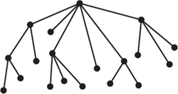
Figure 13.3. A tree.

Figure 13.4. Reducing a planar graph to a single vertex by removing edges a, b, c, d, then e.
There are many proofs of Euler’s formula for graphs. We will give a short one in which, like Cauchy, we remove edges from the graph one at a time. But we will be careful to avoid his mistake.
Begin with any connected planar graph. Pick any edge. This edge either joins two different vertices or it is a loop from one vertex to itself. Suppose the edge joins two vertices. Then shrink the edge until it completely disappears and its two endpoints become one. This can be done so that the resulting graph is planar (see the shrinking of edges a, c, and d in figure 13.4). This procedure decreases the number of edges by one and the number of vertices by one, and it leaves the number of faces unchanged. Thus V − E + F is unchanged. Now suppose that the edge is a loop. In this case, simply remove the edge from the graph (see the removal of edges b and e in figure 13.4). Doing so decreases the number of edges and faces by one, but leaves the number of vertices unchanged. Thus V − E + F is unaltered.
Continue this process of edge removal until a single vertex remains. At this point we have one vertex, no edges, and one face (the exterior region). Thus V − E + F = 2. Because V − E + F was unchanged throughout the process, V − E + F = 2 for the original graph.

Figure 13.5. Two different planar representations of the same graph will have the same number of faces.

Figure 13.6. The complete graphs K1, K2, K3, K4, and K5.
An interesting consequence of this formula is that for a planar graph with E edges and V vertices, every planar representation will have the same number of faces. In other words, if ten people took a planar graph, placed the vertices wherever they desired, and placed the edges on the graph in such a way that no two crossed, all of the graphs would have the same number of faces (F = 1 + E − V, excluding the unbounded face). For instance, in figure 13.5 we have a graph with four vertices and six edges, and we show two planar representations, both of which have three faces.
Because Euler’s formula applies only to planar graphs, we can often use it to prove that a given graph is not planar. To illustrate this idea we introduce two important families of graphs: complete graphs and complete bipartite graphs.
The complete graph with n vertices, denoted Kn, has n vertices and exactly one edge between each pair of vertices. It is the largest possible graph with n vertices that has no loops or parallel edges. The graphs K1 through K5 are shown in figure 13.6. If we removed the loops from the domino graph (figure 11.11), we would have K7.
A relative of the complete graph is the complete bipartite graph. A complete bipartite graph has the property that its vertices can be split into two collections, U and V, such that there are no edges joining vertices in U to vertices in U, no edges joining vertices in V to vertices in V, and exactly one edge joining each vertex in U to each vertex in V. If U has m vertices and V has n vertices, we denote the resulting complete bipartite graph Km,n. The graphs K3,2 and K3,3 are shown in figure 13.7. The typical example of a complete bipartite graph that is found in every introductory graph theory textbook is the utility company graph. The collection U consists of utility companies (gas, water, electric, etc.) and the collection V consists of the customers. Because every customer must have each utility, the graph obtained is a complete bipartite graph.

Figure 13.7. The complete bipartite graphs K3,2 and K3,3.
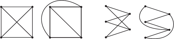
Figure 13.8. K4 and K3,2 are planar graphs.
We would like to determine which complete graphs and which complete bipartite graphs are planar. It is easy to show that K1, K2, K3, K4, Km,1, and Km,2 are planar graphs. For example, in figure 13.8 we see that K4 and K3,2 are planar. It turns out that none of the rest are planar. Using Euler’s formula we will prove that K5 and K3,3 are nonplanar.
To prove that K5 is not planar we use a proof technique called proof by contradiction, or reductio ad absurdum. We assume the opposite of what we need to prove (we assume that K5 is planar) and show that this leads to a logical contradiction. Then we are able to conclude that K5 is not planar. G. H. Hardy wrote, “Reductio ad absurdum, which Euclid loved so much, is one of a mathematician’s finest weapons. It is a far finer gambit than any chess gambit: a chess player may offer the sacrifice of a pawn or even a piece, but a mathematician offers the game.”2

Figure 13.9. An example of a nonplanar graph containing K5.
Suppose K5 is a planar graph. Then we can draw K5 in the plane in such a way that no edges cross. K5 has 5 vertices and 10 edges. Euler’s formula for planar graphs states that V − E + F = 2, thus our planar drawing of K5 must have 7 faces including the unbounded face (because 2 = 5 − 10 + F).
Each edge borders two faces, so 2E = pF where p is the average number of sides on all faces. K5 is a complete graph so it has no loops or parallel edges. Because there are no loops, there are no faces bounded by only one edge, and because there are no parallel edges, there are no faces bounded by two edges. Thus, the average number of edges per face is at least three. So, p ≥ 3, and 2E ≥ 3F . But F = 7 and E = 10 implies that 20 ≥ 21, which is a contradiction. It must be the case that K5 is not planar.
In a similar way we can prove that the complete bipartite graph K3,3 is not planar (give it a try!). The key difference is that because K3,3 is bipartite, a path that begins and ends at the same vertex must have an even number of edges. So there can be no three-sided faces, either.
In general, we have the following theorem.
Kn is not planar when n ≥ 5 and K,m,n is not planar when both m ≥ 3 and n ≥ 3.
It turns out that in some sense K5 and K3,3 are the only obstacles for a graph to be planar. A famous theorem called Kuratowski’s reduction theorem states that the only way a graph can fail to be planar is if it contains a copy of K5 or K3,3 inside it. For instance, the graph shown in figure 13.9 is not planar because it contains a copy of K5.
Next, we give another interesting application of Euler’s formula called Pick’s theorem. It was proved by Georg Alexander Pick (1859–c. 1943) in 1899.3 Pick was an Austrian mathematician who spent much of his life in Prague. He died in the Theresienstadt concentration camp in Czechoslovakia.

Figure 13.10. A polygon formed on a geoboard.
To introduce Pick’s theorem we turn to the geoboard, a popular teaching tool invented by Caleb Gattegno (1911–1988) that gives children a hands-on way of learning basic geometry. A geoboard can be made at home by hammering nails halfway into a wooden board so that they form a square grid. The students can wrap rubber bands around the nails to form polygons (see figure 13.10). The teacher can then discuss geometric concepts such as perimeter, angle, area, and the Pythagorean theorem.
Pick’s theorem gives a very easy way to compute areas of even the most complicated nonconvex polygons (we do insist, however, that the rubber band not cross itself).
PICK’S THEOREM
If there are B nails on the boundary of the polygon and I nails in the interior of the polygon, then the area is A = I + B/2 −1.
For instance, because the polygon in figure 13.10 has B = 12 and I = 5, the area is 5 + 12/2 − 1 = 10.
It turns out that at least one forester in Oregon used an approximation of Pick’s theorem to estimate the size of his forest.4 The forester took a transparency with a lattice pattern of dots on it and placed it on a polygonal map of his land. To estimate the area he added the number of dots in the interior to half the number on the boundary (very nearly Pick’s theorem!) and multiplied this by the appropriate scaling factor.
Pick’s theorem is an elementary consequence of Euler’s formula once we know the area of a primitive triangle. A triangle is primitive if it has no nails in its interior and boundary nails only at the vertices (such as the shaded triangle in figure 13.11). In other words, a triangle is primitive if B = 3 and I = 0. Surprisingly, every primitive triangle has area 1/2.

Figure 13.11. The parallelogram formed from a primitive triangle tiles the plane.
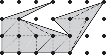
Figure 13.12. The polygon is triangulated into primitive triangles.
Unfortunately, this fact is somewhat tedious to prove. Instead of giving the proof we will give an indication of why it is true. It is easy to see the plane (an infinite geoboard) can be tiled by 1 × 1 squares. These tiles have the property that if they are shifted one unit up, down, right, or left, they will land on another square. Likewise, take the primitive triangle and extend it to form a parallelogram with double the area (see figure 13.11). Like the square, the parallelogram can tile the plane by repeatedly moving it one unit to the left, to the right, up, and down. So, like the square, the parallelogram has area 1. Thus the triangle has area 1/2.
We are now able to prove Pick’s theorem. First, triangulate the polygon into T primitive triangles (such as in figure 13.12). If we count the unbounded region as a face, then F = T + 1. Because every triangular face has area 1/2, the total area of the polygon is A = (1/2)T.
Every bounded face has three sides, so the quantity 3T counts each edge twice except for the edges along the boundary, which are counted once. Because the number of edges on the boundary is the same as the number of vertices on the boundary, we have
3T = 2E − B,
or, solving for E,
![]()
The number of vertices is V = I + B. Applying Euler’s formula we have,
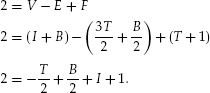
So, the number of triangular faces is
T = 2I + B − 2,
and the total area is given by
![]()
as claimed.
We end with two pencil-and-paper games. Despite their similarities, one is an intellectual challenge and the other a hoax on the players with the outcome determined before the first move.
According to Martin Gardner (b. 1914), the long-time mathematics columnist for Scientific American, the game of “sprouts” was invented at teatime one February afternoon in 1967 by John Horton Conway (b. 1937) and Michael Paterson at the University of Cambridge. It became an underground sensation. Conway wrote to Gardner that “the day after sprouts sprouted, it seemed that everyone was playing it. At coffee or tea times, there were little groups of people peering over ridiculous to fantastic sprout positions.”5
The game begins with any number of dots on a blank sheet of paper. The first player draws a curve from one dot to another dot or back to itself, then places a new dot somewhere along the curve. Play alternates with both players drawing a curve from dot to dot and placing a new dot along the way. The only rules are that a new curve cannot pass through an existing curve or dot and that at most three lines can meet at any dot. The winner is the last player able to make a move. Figure 13.13 shows a 2-dot game in which player 2 wins in the fourth move.
The more dots at the outset, the longer the game, but the game cannot go on forever. At the start of an n-dot game there are 3n available places to attach edges. Each time a new edge is drawn, the number of open spots decreases by one (two are used up, one is added). So the longest the game could possibly last is 3n − 1 moves.
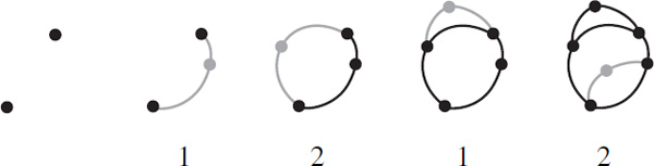
Figure 13.13. Player 2 wins this game of sprouts.

Figure 13.14. Player 2 wins this game of Brussels sprouts.
As it turns out, for small values of n there is a slight advantage to going either first or second, depending on the number of dots. If the game starts with 2 dots, the second player can always make choices that guarantees a win. The same is true for n = 1, 6, 7, and 8 dots. On the other hand, the first player has the advantage for n = 3, 4, 5, 9, 10, or 11 dots. Most of these cases (n > 6) were checked by computer.6 For larger n values it is not known if either player has an advantage. Although there is a theoretical unfairness in this game, for all but the smallest of n-values the winning strategy is unknown. So in practice, it is still an intellectual challenge to win the game.
Later Conway invented a variant of sprouts that he dubbed “Brussels sprouts.” Instead of starting with n dots, the game begins with n plusshaped crosses. Each turn a player joins two free arms with a curve and puts a new plus sign (producing two free arms) in the middle of the edge (see figure 13.14). Unlike sprouts, the rules for Brussels sprouts allow four edges to meet at the same location. As before, the winner is the last player able to make a move. It turns out that the humorous name Brussels sprouts was a tip-off that the game itself was a joke.

Figure 13.15. The final graph for the game of Brussels sprouts in figure 13.14.
We saw that a game of sprouts must end, but this is not so obvious in Brussels sprouts. Each move destroys two free arms and adds two more, so it seems the game could go on forever. However, every game of Brussels sprouts is destined to end, and herein lies the joke. Regardless of how clever or dim the players, the game will always last for exactly 5n − 2 turns. In other words, an odd number of starting crosses guarantees the first player to be the winner, and an even number guarantees victor’s spoils to the second player.
If we ignore the free arms, then at each turn, the game board is a planar graph (perhaps having several connected components). If we take each cross to be a vertex, then each move adds two edges and one vertex. Unless the new curve joins two connected components, each move also adds a face.
We claim that play will stop when the graph is connected and has exactly 4n faces (counting the exterior region as a face). At the start of the game there are n crosses having 4n free arms. Because each play wipes out two free arms and adds two more, there are always 4n free arms. Each region must have at least one free arm pointing inside it, namely the one coming from its most recently drawn boundary curve. So the graph can have at most 4n faces. On the other hand, if there are fewer than 4n faces, then some region must contain two free arms, and the game is not yet over.
Suppose the game ends after m turns, leaving a connected graph with V vertices, E edges, and F = 4n faces. (The final configuration in figure 13.15 has V = 10, E = 16, and F = 8.) As we explained earlier, each of the m turns adds two new edges and one new vertex. Because the game began with no edges and n vertices, at the end of the game there are E = 2m edges and V = n + m vertices. Now we use Euler’s formula to obtain
2 = V − E + F = (n + m) − 2m + 4n.
Solving form gives m = 5n − 2.
So, if you feel the need to swindle your unsuspecting friends, ask them to play Brussels sprouts. Give them the choice: they can choose who goes first or the number of starting crosses. Either way, you can guarantee that you are the winner.