CHAPTER 19

COMBING THE HAIR ON A COCONUT

Let chaos storm!
Let cloud shapes swarm!
I wait for form.
—Robert Frost, “Pertinax”¹

Many scientists use mathematics as a tool to predict behavior. A scientist may have an equation or a system of equations that describes the interactions of the quantities in their model. Then they use mathematics to draw conclusions from these equations.

Often the mathematical models are differential equations. These describe the rates of change of various quantities as a function of time. For example, an ecologist might use a system of differential equations to model the population dynamics of rabbits and foxes living in a wildlife refuge driven by their predator-prey relationship. When the number of rabbits is large, the foxes have an abundant food supply. As the foxes feed on the rabbits, the number of foxes increases and the number of rabbits decreases. Eventually, the foxes’ food supply dwindles, causing their population to decrease. This, in turn, allows the rabbits to prosper again. We see this cyclic behavior illustrated visually in figure 19.1.

Differential equations are expressed as an algebraic relationship among variables and their derivatives. By a solution to a differential equation, we mean that for a given initial condition we can predict the future behavior of the system. In other words, if we know how many rabbits and foxes there are today, we can predict how many there will be a year from now. The curve in figure 19.1 is the plot of a solution curve. The arrows indicate the direction of positive time. The curve is plotted in the phase space, a topological object representing all possible values of the variables. In this case the phase space is the first quadrant of the plane (since the numbers of number of rabbits rabbits and foxes must be nonnegative). In more exotic examples the phase space may be a more complicated topological shape.

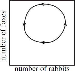
Figure 19.1. The predator-prey model.

Sometimes finding a particular solution to a differential equation is not sufficient for the scientist. It is often more important to draw qualitative conclusions. Does the system have an equilibrium—populations for which the death rate equals the birth rate for both species? Are there initial conditions that lead to extinction of either or both species? To a population explosion? Will the populations exhibit a cyclic behavior, or will they vary chaotically? Even though we may be able to solve a differential equation using calculus, it may not be easy to answer these important “global” questions.

In order to better understand the solutions of a system of differential equations, we may wish to come up with a more visual, geometric way to represent them. The two common techniques are to produce a flow or a vector field in the phase space. A flow, also known as a continuous dynamical system, associates to each point in the phase space the trajectory for the point to move. This trajectory is simply the solution curve for the differential equation. Several flow lines for the predator-prey model are shown in figure 19.2. They show that for any nonequilibrium pair of initial populations, the populations rise and fall cyclically.

Instead of expressing a differential equation algebraically or as a flow, we may describe it in terms of a vector field. In contrast to scalar quantities such as temperature, time, brightness, or mass, which can be described by the magnitude alone, vector quantities have a magnitude and a direction. In physics one might use a vector to describe velocity; the vector points in the direction of motion and the magnitude of the vector represents the speed at which the object is traveling. We could give other examples, but velocity is probably the most intuitive. In fact, if we think of a flow as the motion of particles, then the vectors in the vector field are the velocity vectors for the particles in the phase space.

Figure 19.2. The associated flow and vector field for the predator-prey model.

In figure 19.2 we see that there is a single point of equilibrium—a point where the numbers of foxes and rabbits remain unchanged in time. The vector at this point of equilibrium has magnitude zero, so we say that vector field has a zero at this point. Equivalently, the flow here has a fixed point or rest point. Zeros of vector fields are often of great importance because they represent equilibrium points of the system.

We devote the rest of the chapter to an investigation of vector fields on surfaces and not to the differential equations from which they came. Our primary goal is to understand the relationship between the zeros of a vector field and the topology of the surface.

One of the easiest ways to obtain a vector field on a surface is to place the surface in 3-dimensional space and have the vectors “point downhill,” and the steeper the descent, the longer the vector. This is called a gradient vector field. In figure 19.3 we show the gradient vector field for a sphere and a torus. One way to think about the flow associated to the vector field is to imagine the surface covered by molasses. The flow lines are simply the paths of the viscous syrup as it oozes down the surface.

As we see in figure 19.3, the gradient vector fields on the sphere and the torus have zeros—the sphere has two (one at the north pole and one at the south pole) and the torus has four (at the top and bottom of the torus and at the top and bottom of the hole). Must every vector field on the sphere have a zero? Must every vector field on the torus have a zero? If we can answer such a question “yes” for some surface S, then we have a powerful result. It says that any time the phase space of a system is S, it must have a point of equilibrium.

Figure 19.3. Gradient vector fields for a sphere and a torus.

Figure 19.4. Vector fields near a zero and their corresponding flows.

As a partial answer to these questions, we have the beautiful Poincaré-Hopf theorem. It establishes a surprising relationship between the zeros of a vector field and the Euler number. In order to understand the theorem we must look a little closer at zeros of vector fields.

Not all zeros are the same. In figure 19.4 we see five different zeros and their corresponding fixed points for the flow. The behaviors in the neighborhood of the zeros are all very different. A source repels all nearby points, a sink attracts them, a saddle does both, all points near a center flow around the fixed point, and points near a dipole flow away and then back again (resembling the magnetic field lines of a bar magnet).

Sources, sinks, and saddles often arise as zeros of the gradient flow. In figure 19.5 we see that a source appears at the top of an overturned bowl, a sink at the bottom of a bowl, and a saddle from the middle of a saddle-shaped surface. Notice that in figure 19.3 the gradient flow on the sphere has one source and one sink, and the gradient flow of the torus has one source, one sink, and two saddles.

Figure 19.5. A source, a sink, and a saddle in a gradient vector field.

Our intuition tells us that sinks, saddles, and sources are somehow distinct and that there must be a rule that governs the number of each type of zero. We see from the gradient-flow example that a sphere can have a vector field with two zeros, but it is difficult to imagine a vector field on the sphere with one sink and one saddle. The key idea that we need to distinguish zeros is the index.

We compute the index of a zero as follows. Draw a small circle around the zero. The only conditions that this circle must satisfy are that (1) it must contain only one zero, and (2) it must be the boundary of a disk (for example, such a circle on torus cannot go around the tube or the central hole). Now place an imaginary dial at some point on the circle. The hand of the dial should point in the same direction as the vector field. (If the vector field represented the direction of a magnetic field, then we could use a compass as the dial.) As we move the dial around the circle, the hand of the dial turns. Move the dial around the circle one time counterclockwise. Each time the hand turns once counterclockwise, add one to the index, and each time it turns once clockwise, subtract one from the index. The index is often called the winding number of the vector field around the zero.

Consider the sink in figure 19.6. We see the dial in eight locations around the circle. As the dial traverses the circle once counterclockwise, the hand turns once counterclockwise. So the index of a sink is 1. For the saddle, the hand turns once clockwise as the dial follows the circle around the zero once counterclockwise. So the index of a saddle is −1. In a similar manner we can compute the indices of the other zeros in figure 19.4. The sink and the center have index 1, whereas the dipole has index 2.

Figure 19.6. A sink has index 1 and a saddle has index −1.

Figure 19.7. The index of a saddle is 2(−1) + 1 = −1 and the index of a sink is 6(-1) + 7(1) = 1.

We now give a second way of computing the index of the zero of a vector field. This approach will be useful to us later. Suppose we put the zero in the interior of a polygonal face (it is acceptable to have curved edges). We are free to chose any polygon as long as a few criteria are satisfied. As before, we must choose the polygon so that our zero is the only zero in the polygon and the polygon must bound a disk. In addition, we insist that every vector that lies on an edge points either inward or outward. We do not want a vector to point along an edge. (Such a polygon always exists, although this is not obvious.) In figure 19.7 we see a saddle placed inside a square and a sink inside a hexagon in such a way that all vectors are either pointing inward or outward.

Figure 19.8. Three vector fields on the sphere.

We now single out those edges and vertices on which the vector field is pointing inward. Along each such edge place a −1, and along each such vertex place a 1. Finally, put a 1 in the middle of the polygon. It turns out that the sum of all these numbers is the index of the zero. We see that this is true for the saddle and the sink in figure 19.7.

At last we are able to state the Poincaré-Hopf theorem. It gives us a topological way to determine whether a vector field has a zero (or equivalently, a flow has a fixed point). It also gives us insight into the relative numbers of each type of zero on a particular surface.

Before proving this theorem, we will give some examples. In figure 19.8 we see three different vector fields on the sphere. The first, the gradient vector field, has a sink and a source (each with index 1), the second has two centers (each with index 1), and the third has one dipole (with index 2). In all three cases the indices sum to 2, the Euler number of the sphere.

Earlier we saw that the gradient vector field on the torus (figure 19.3) has four zeros—one source, two saddles, and one sink. The sum of their indices is 1 + 2(−1) + 1 = 0, the Euler number of the torus.

As an added bonus, gradient vector fields enable us to compute the Euler number of surfaces without drawing vertices, edges, and faces. In figure 19.9 see the sphere placed in a bent U-shape. The gradient vector field has two sources, one saddle, and one sink; thus the sum of the indices is 2(1) + 1(−1) + 1(1) = 2. The double torus has one source, four saddles, and one sink, so χ(double torus) = 1 + 4(−1) + 1 = −2. The Klein bottle has a source, two saddles, and a sink, so χ(Klein bottle) = 1 + 2(−1) + 1 = 0. We summarize this situation as follows:

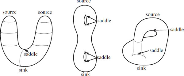
Figure 19.9. The Euler numbers of a sphere, a double torus, and a Klein bottle are 2, −2, and 0, respectively.

The Poincaré-Hopf theorem states that if a vector field on a surface has finitely many zeros, then the sum of the indices is the Euler number. From this we conclude that if a vector field has no zeros, then the Euler number of the surface must be zero. So any vector field on a surface with nonzero Euler number must have at least one zero! The Euler number of the sphere is 2; so every vector field on a sphere must have a zero. This famous theorem, first proved by L. E. J. “Bertus” Brouwer (1881–1966) in 1911,² has the memorable name the hairy ball theorem. It is so-named because if we think of a hairy ball (a tennis ball or a hedgehog) as a sphere with a vector field, then it is impossible to comb it without introducing a cowlick. It is also said that “you can’t comb the hair on a coconut.”

From this theorem we can draw the conclusion mentioned in the introduction: that there is always a location on earth where there is no wind. If we view the earth as a sphere, then the surface winds yield a vector field. By the hairy ball theorem, there is a spot on earth where that vector field is zero. The example shown in figure 19.10 has a point of no wind in the center of a cyclone off the coast of South America. (Actually, because this zero has index 1, there must at least one more windless spot on the other side of the earth!)

Figure 19.10. Wind vectors on the surface of the earth.

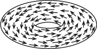
Figure 19.11. A vector field with no zeros on the torus.

Because the Euler number of the torus is zero, the Poincaré-Hopf theorem does not guarantee that every vector field has a zero. Indeed, in figure 19.11 we see an example of a nonvanishing vector field on the torus.

The hairy ball theorem is an example of an “existence theorem.” They are ubiquitous in theoretical mathematics. They are simultaneously very powerful and frustratingly imprecise. On the one hand, given only a simple set of hypotheses (a vector field on a sphere), we can make the confident assertion of the existence of some object (a zero vector). However, it is often the case that neither the statement nor the proof of an existence theorem gives a technique for finding this object. We know there is another windless location on the other side of the globe in figure 19.10, but it could be anywhere, and moreover, there may be one or there may be one or there may be many. It is like searching for a child’s misplaced teddy bear at bedtime—you know it is in the house, but it could be anywhere—under the bed, in the closet, or in the microwave oven. Although more techniques need to be employed to find these objects, often the existence of the object is sufficient for the purpose at hand.

Figure 19.12. Henri Poincaré.

The Poincaré-Hopf theorem is named after the two mathematicians who contributed most to its development, although several others made important contributions as well.

Henri Poincaré was born in Nancy, France, in 1854 into a well-respected upper-middle-class family (his first cousin Raymond Poincaré would later become the president of the French Republic).

Henri’s mathematical talent became clear early, with one of his teachers calling him a “monster of mathematics.”³ He began making important contributions to mathematics while still in his twenties, and was elected to the Académie des Sciences at the age of thirty-three. He was the stereotypical mathematical genius; he was clumsy, had poor vision, was absent minded. He also possessed a supreme intellect and had the ability to retain and juggle many abstract concepts in his head.

Poincaré is generally acknowledged as the preeminent mathematician of his era. He was the last great universalist. Like Euler and Gauss, Poincaré was an expert in nearly every area of mathematics, pure and applied. He was a voracious reader who was familiar with the latest results. Also like Euler (but unlike Gauss), Poincaré published extensively. He penned nearly five hundred articles, as well as many books and sets of lecture notes. He made important and lasting contributions in such diverse fields as function theory, algebraic geometry, number theory, ordinary and partial differential equations, celestial mechanics, dynamical systems, and, of course, topology. He also published many articles in theoretical physics. Poincaré had a restless curiosity that kept him moving from topic to topic. He would attack a new area of mathematics, make an indelible mark, then move on to the next. A contemporary called him “a conqueror, not a colonist.”

It is remarkable that not only was he able to produce the highest-level mathematics, he was also able to write at a level accessible to nonspecialists. He wrote numerous lucid and fascinating publications about science and mathematics for a lay audience. His writings were widely read and translated into many languages.

Poincaré’s expertise spanned all of mathematics, but throughout his career he kept returning to the study of differential equations. His successes in this area were profound. According to the mathematician Jean Dieudonné (1906–1992), “The most extraordinary production of Poincaré . . . is the qualitative theory of differential equations. It is one of the few examples of a mathematical theory that sprang apparently from nowhere and that almost immediately reached perfection in the hands of its creator.”⁴ The prime example was his discovery of the index formula.

His first contribution was in 1881. In this work, he took a differential equation and produced a vector field on the sphere. He defined the index of a zero and proved that the sum of the indices of all zeros is 2.⁵ Of course, it is no coincidence that the sum equals 2, for that is the Euler number of the sphere. Poincaré made this observation precise in 1885 when he proved that the sum of the indices of a vector field on a surface is the Euler number of the surface.⁶ The following year he defined an index for zeros of a vector field in n-dimensional space, and he sketched the idea of an n-dimensional index theorem. The difficulty in following through with this program was that the topological machinery did not yet exist (this, as we will see in chapter 23, Poincaré would later create).

In 1911 Brouwer properly generalized Poincaré’s index theorem to the n-dimensional sphere, Sⁿ. We are familiar with S¹, the unit circle in the plane (x² + y² = 1), and S², the unit sphere in 3-dimensional space (x² + y² + z² = 1). More generally, Sⁿ is the collection of points 1 unit away from the origin in (n + 1)-dimensional space . Brouwer proved that for any vector field on Sⁿ, the sum of the indices of the zeros is 0 if n is odd and 2 if n is even.⁷ In chapters 22 and 23 we will discuss the Euler number in higher-dimensional spaces. When we do, we will discover that χ(Sⁿ) = 0 when n is odd and χ(Sⁿ) = 2 when n is even.

Figure 19.13. Heinz Hopf.

The next major contributor was Heinz Hopf (1894–1971). Hopf was born in Breslau, Germany (now Wroclaw, Poland). His work in topology made a profound impact on twentieth-century mathematics. A student of Hopf’s wrote, “Hopf selected deep problems with an unerring instinct and let them mature. Then he presented in one piece a solution that showed new thoughts and methods.”⁸

In his memoirs Hopf pinpoints the pivotal moment in his mathematical career as a two-week period in 1917 when he was on leave from his military service during World War I. He sat in on a mathematics class at the University of Breslau during a presentation of a topological theorem of Brouwer’s. After serving on the Western Front, being wounded twice, and receiving the Iron Cross, he resumed his study of mathematics at the University of Breslau. His mathematical career took him to several German universities, Princeton University, and finally to Eldgenössische Technische Hochshule (ETH) in Zurich, Switzerland.

Two years after he arrived in Switzerland, the Nazi party came to power in Germany. Although he was raised Protestant, his father was born Jewish. Solomon Lefschetz and others at Princeton urged Hopf to return, but he and his wife refused to leave Switzerland, and instead worked to help refugees from Germany. Eventually the German government threatened to revoke his citizenship if he did not return. Reluctantly, he gave up his German citizenship and became Swiss. After the war Hopf remained in Switzerland and worked diligently to reestablish mathematics in Germany.

Of Hopf’s many important contributions to topology, some of the first were on the topology of vector fields. Beginning in 1925 he published a series of papers generalizing Poincaré’s index theorem.⁹ We stated the Poincaré-Hopf theorem for surfaces, but Hopf proved that it applies to higher-dimensional generalizations of surfaces, called manifolds (we will learn more about manifolds in chapter 22).

Although the Poincaré-Hopf theorem is usually stated for closed surfaces, mathematicians discovered various generalizations of the theorem. There is an extremely general version for surfaces with boundary,¹⁰ but we will state the following simpler version.

The hairy ball theorem does not apply to hair on our heads because the hair-covered region of our head is not topologically a sphere—it is a disk. Indeed, the “slicked-back” and “ponytail” styles have no cowlick. However, on a “crew cut” head we see the roots of a person’s hair often grow away from the center of the head—downward in the back, toward the ears on the sides, and into the face from the front. Because this hairy vector field points outward along the boundary, the sum of the indices of the zeros must equal χ(disk) = 1. So there must be a cowlick. The author’s baby daughter (whose hair is still just peach fuzz) has the beginnings of three cowlicks, two outward spirals (each of index 1) with a saddle between them (index −1).

We now sketch a proof of the Poincaré-Hopf theorem for surfaces without boundary. (It is not difficult to modify this proof to handle the surfaces with boundary.) The proof is based on one by William Thurston (b. 1946).¹¹

We begin with a carefully chosen partition of the surface. First, put each zero of the vector field inside its own polygonal face. These faces can have any shape, with any number of sides, as long as no vector that lies on an edge is parallel to the edge. That is, every vector on the boundary of the face must point in or out.

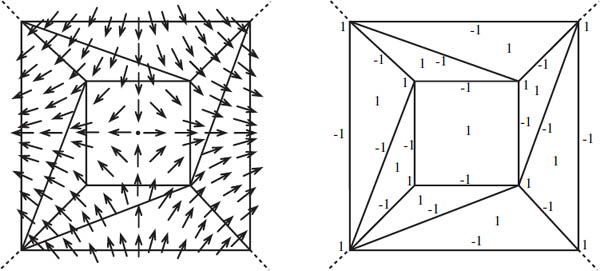
Figure 19.14. A partition of a surface with at most one zero in each face, and the vertices, edges, and faces labeled accordingly.

At this point we have faces enclosing all of the zeros of the vector field. Complete the partition by triangulating the rest of the surface. We can do this in any way that we want, although, just as with the earlier faces, we insist that all vectors on the boundaries of the triangles point inward or outward, not along the edge (see figure 19.14).

Now, place a 1 on each vertex, a −1 on each edge, and a 1 in the middle of each face. So when we add all of these quantities over the entire surface, we will obtain V − E + F, or in other words, χ(S). More specifically, because each edge bounds two faces and the vector field points into one of these two faces, put an edge’s −1 in the face into which the vectors point. Similarly, each vertex is located at the junction of several faces, but there is one face into which the vector points. Put the 1 in this face (see figure 19.14).

First we examine the triangular faces that do not contain zeros of the vector field. As we see in figure 19.15, there are only two possible situations. One is that the vectors point inward on one edge and no vertices. The other is that the vectors point inward on two edges and on the vertex between them. In either case, the sum of the 1s and −1s is zero. Hence, these triangular faces contribute nothing to the Euler number.

On the other hand, recall that for the faces containing a zero, this technique can be used to compute the index. So each face that contains a zero contributes to the sum a value equal to the index of the zero. As claimed by the Poincaré-Hopf theorem, the sum of all the 1s and −1s is equal to both the Euler number and to the sum of the indices of the zeros.

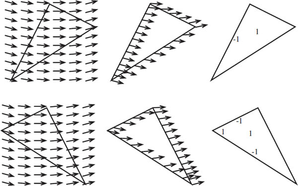
Figure 19.15. The triangles containing no zeros contribute nothing to the Euler number.

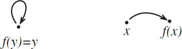
Figure 19.16. The point y is a fixed point for f and x is not.

As stated, the Poincaré-Hopf theorem is a theorem about vector fields, but because vector fields can be used to construct flows, it can also be interpreted as a fixed point theorem for continuous dynamical systems. We conclude this chapter by mentioning another famous fixed point theorem.

A flow on a surface is a mathematical way of describing the continuous movement of particles. We now look at a related, but quite different situation. Suppose that instead of flowing, each point in a surface S jumps to a new location. Mathematically, we describe this motion using a continuous function f with domain S and range S (by continuous we mean simply that nearby points jump to nearby points). A point begins at a point x, then it moves to a new point f(x). Just as for flows, we are especially interested in those points that do not move. A point y in S is called a fixed point for f if f(y) = y (see figure 19.16).

Probably the most famous fixed point theorem is the Brouwer fixed point theorem. It applies to continuous functions from the n-ball to itself.

Figure 19.17. The vector field for a function from B² to itself.

The n-ball, denoted Bⁿ, is the set of all points in n-dimensional space that are within one unit of the origin. That is, it is the set of points satisfying or simply, Bⁿ is the set of points contained inside the (n − 1)-dimensional sphere, Sⁿ⁻¹. Brouwer proved the result for B³ in 1909¹² and for Bⁿ (n > 3) in 1912.¹³

Here is one way to think about this remarkable theorem. Consider the case n = 2. B² is a disk in the plane—the region enclosed by S¹, the unit circle. Imagine that it is a dinner plate. Cover the plate with a piece of paper that is at least as large as the plate, then cut the part of the paper that hangs off the edge of the plate. Now, pick up the paper, crush it into a ball (being careful not to rip it), and place it back on the plate. The Brouwer fixed point theorem says that some part of the paper is over exactly the same spot that it was originally. This same reasoning says that a designer of a one-story shopping mall can place a map of the mall anywhere in the building and be able to put a star on the map labeled “you are here.”

The proof of this theorem follows easily from the Poincaré-Hopf theorem (the version for surfaces with boundary). We will consider the case when n = 2, but the argument for larger n is identical. Begin with a function f from B² to itself. Define a vector field on B² as follows: to each point x in B² assign the vector that has its tail at x and tip at f(x) (see figure 19.17). B² is a surface with boundary and all vectors on the boundary point inward, so we may apply the Poincaré-Hopf theorem. Because χ(B²) = 1 ≠ 0, the vector field must have at least one zero. In this case, a zero vector corresponds to a point y for which f(y) = y. In other words, f must have at least one fixed point.

In fact, the Brouwer fixed point theorem applies equally well to any shape that is homeomorphic to Bⁿ. The coffee in a coffee cup is homeomorphic to B³. Swirl the coffee vigorously in the cup (without spilling it!), and according to the Brouwer fixed point theorem, after it comes to rest, there is a molecule of coffee in precisely the same location as it was at the start.

In this chapter we observed that the topology of an object, measured simply by its Euler number, can force global behavior that does not appear to have any relationship to the global topology—the existence of fixed points of flows or functions. As we will see in the next two chapters, the topology of a shape can also determine certain of its global geometric properties.