CHAPTER 21

THE TOPOLOGY OF CURVY SURFACES

If others would but reflect on mathematical truths as deeply and as continuously as I have, they would make my discoveries.
—Carl Friedrich Gauss¹

One of the most fundamental topics in the geometry of planar curves is curvature. The curvature at a point x is a number, k, that measures the “sharpness” of the turn at x—it measures how quickly the tangent vectors change direction. Roughly speaking, given a normal vector to a curve at x, if the curve bends in the direction of , then k > 0, if it bends away, then k < 0, otherwise k = 0 (see figure 21.1). The more sharply it bends, the larger (in absolute value) k is.

By the Jordan curve theorem a simple closed curve in the plane has an inside and an outside. So we can pick normal vectors along the entire curve, having them all point toward the inside. Then we can compute the curvature at each point on the curve. Typically, the curvature varies from point to point (see figure 21.2). It is possible to sum the curvature over the entire curve to obtain the total curvature. The details of this computation are beyond the scope of this book, but a calculus student should recognize that because the curvature varies continuously, the sum in question is the integral of the curvature. We have the following theorem.*

In other words, the total curvature is the same number for all smooth simple closed curves! If we took a loop of string and dropped it on a table so that it did not cross itself, then the regions of negative curvature would cancel with regions of positive curvature, so that in the end, the total curvature is 2π. That is, being homeomorphic to a circle completely determines the total curvature. Again we see how topology controls geometry.

Figure 21.1. Curves with k > 0, k < 0, k = 0, and k = 0 (left to right).

Figure 21.2. A curve with regions of positive, negative, and zero curvature for normal vectors pointing toward the inside.

We will not prove this theorem, but it is closely related to the theorem of turning tangents from the previous chapter. Again, a calculus student sees that because we are summing the rate of change of the turning tangents, the total curvature is just the total change in the turning tangents, or 2π.

We can also think of this theorem as another generalization of the exterior angle theorem for polygons. A polygon has no curvature along its sides, instead it carries all of its curvature at the corners in the form of the exterior angles. The total curvature is 2π.

Now we turn our attention from curves to surfaces. Because we are studying the geometric properties of surfaces, we must assume that the surfaces are rigid, and not made of rubber as were our topological surfaces. We assume that they are smooth, with no sharp creases or corners.

Just as we did with curves in the plane, we investigate the curvature of surfaces in 3-dimensional space. Again, pick a normal vector to the surface at a point x. Then look at a plane that passes through the point x and is parallel to . The intersection of the surface and the plane is a curve, so we can compute its curvature. Typically the curvature of these curves will be different for different planes through x. The largest and smallest values, k₁ and k₂, respectively, are called the principal curvatures of the surface at x (see figure 21.3). In 1760 Euler proved that the principal curvatures arise from perpendicular planes.²

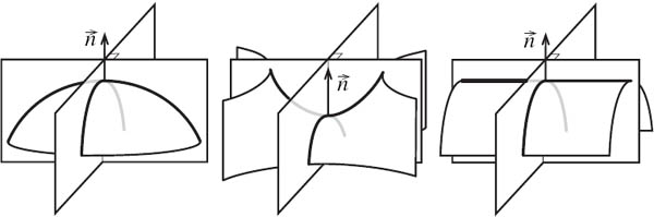
Figure 21.3. Surfaces for which k₁, k₂ < 0 (left), k₁ > 0, k₂ < 0 (middle), and k₁ = 0, k₂ < 0 (right)

It was in this way that geometers measured the curvature of surfaces until Gauss made a simple, but crucial modification. He multiplied the principal curvatures to form a single curvature value, now called Gaussian curvature: k = k₁k₂ This seemingly trivial operation, which appears to contain less information than do the two principal curvatures separately, produced an important numerical value that helped mathematicians understand the curvature of surfaces.

Surprisingly, most great mathematicians were not child prodigies; their genius needed to grow and mature, only coming out later in life. However, it was clear from a young age that Gauss had tremendous mathematical ability. He was born in 1777 in Brunswick, Germany. At only three-years old Gauss shocked his father, Gerhard, when he pointed out an error in his father’s arithmetic in his financial books. On subsequent Saturdays Gauss would sit in a highchair and assist his father.

In his old age Gauss enjoyed telling how, when he was seven-years old, he shocked one of his brutish and overbearing school teachers. The teacher asked the class to sum an arithmetic series (1 + 2 + 3 + . . . + 100, for the sake of the story³). Gauss almost immediately wrote the number 5050 on his slate tablet, which he placed on the table in front of the skeptical teacher, and announced “ligget se” (there it lies). Instead of performing the tedious summation, Gauss noticed that by adding the first number to the last, the second to the penultimate, and so forth, each sum would be 101 (i.e., 1 + 100, 2 + 99, 3 + 98, . . . ). Because there are fifty such pairs, the total must be 50.101 = 5050.

Figure 21.4. Carl Friedrich Gauss.

This classroom incident set in motion a chain of events that in 1791 brought Gauss to the attention of Carl Wilhelm Ferdinand, Duke of Brunswick. The Duke was taken with the fourteen-year-old boy and promised to pay for his schooling. The generous Duke financed Gauss’s education at the Collegium Carolinium and University of Göttingen, and continued to pay his salary until the Duke’s death at the hands of Napoleon’s army in 1807.

The Duke’s instinct about the boy was correct. Gauss’s first important result, the proof of the quadratic reciprocity law, came when he was nineteen-years old. This theorem, which he called theorema aureum (the golden theorem), had eluded both Euler and Legendre.

Gauss chose as his seal a tree bearing a few pieces of fruit with the words pauca sed matura (few, but ripe). Indeed, this motto perfectly embodies Gauss’s career. Unlike the prolific Euler, Gauss was not quick to publish. He never published trivialities, insisting that each publication be a masterpiece. As he said, “You know that I write slowly. This is chiefly because I am never satisfied until I have said as much as possible in a few words, and writing briefly takes far more time than writing at length.”⁴ Among the many fields upon which Gauss left his mark were astronomy, geodesy, theory of surfaces, conformal mappings, mathematical physics, number theory, probability, topology, differential geometry, and complex analysis.

Figure 21.5. A surface (torus) with variable curvatrure: positive, negative, and zero. Other surfaces have constant positive curvature (sphere), zero curvature (cylinder), and constant negative curvature (pseudosphere).

Because of his drive for perfection, he left many great results unpublished. His mathematical diary (Notizenjournal), which was discovered forty-three years after his death, contains a wealth of mathematics. Had Gauss published some of these results and nothing else, he would have been remembered as an influential mathematician. It is frustrating to realize that mathematicians toiled for years only to rediscover ideas that had been known to Gauss. One wonders how much further nineteenth century mathematics would have progressed had Gauss been more willing to publish his results.

After the Duke died, Gauss was forced to take a position as the director of the Göttingen Observatory. He spent much of the last twenty years of his life dealing with astronomical affairs at the observatory. He lived to the age of 78, passing away peacefully on February 23, 1855.

Using Gauss’s single-valued approach to measuring curvature, k = k₁k₂, we can say that the curvature at a point is positive, negative, or zero. Returning to figure 21.3, we see that if like the bottom of a bowl, both curves bend toward (or both curve away from) the normal vector, then the signs of k₁ and k₂ are the same, and we have a positive curvature. On the other hand, if like a saddle, one curve bends toward the normal vector and one away, the signs of k₁ and k₂ are opposite, and the curvature is negative. If one or both of the principal curvatures are zero, as with a cylinder or a plane, the curvature is zero.

It is important to emphasize that curvature is measured at a single point. A typical surface will have regions of positive, negative, and zero curvature. For instance, the torus in figure 21.5 has positive curvature in the region farthest from the center, negative curvature in the region nearest the center, and zero curvature on the boundary between these two regions. There are surfaces with constant curvature. A sphere (not a topological sphere, but an actual sphere) has constant positive curvature, and a plane and a cylinder have zero curvature. The most famous example of a surface with constant negative curvature is the trumpet-shaped surface known as the pseudosphere, so-named not because of a resemblance to a sphere, but because of its constant curvature.

Gaussian curvature, area, and angle excess are intimately related quantities, and it is their relationship that we must understand. We have already seen that curvature and angle excess are related. Figure 20.9 shows a geodesic triangle on a sphere with an angle excess and one on a saddle with an angle deficit. The flatter a surface, the more it resembles a plane, and the more a triangle looks like a planar triangle. Positive curvature yields an angle excess and negative curvature causes an angle deficit.

It should also be clear that size matters. Triangles that are very small experience very little of the surface’s curvature (think of two equilateral triangles on the earth, one which has sides 1,000 miles long and one which has sides 1 inch long). As we zoom in to a surface, it looks more and more flat. The smaller the triangle, the closer the angle excess is to zero.

Here is another illustration that curvature and area are related. Suppose we took a portion of a positively curved surface, like a piece of onion skin or a cabbage leaf. If we tried to flatten it out on a table, we would find that there is too much area in the middle. Undoubtedly, the outside edge of the onion skin would rip as we tried to press it flat. This is why in the usual (Mercator) projection of the earth, Greenland dwarfs the continental United States, when in fact three islands the size of Greenland could fit comfortably inside the lower forty-eight states. We run into the opposite problem for negatively curved surfaces. If we were to cut a portion from a saddle-shaped surface there would be too much area at the extremes to flatten the disk onto a table. The outside edge of the disk would fold and wrinkle.

We can exploit the relationship among curvature, area, and angle excess to obtain an alternate definition of Gaussian curvature. Consider a geodesic triangle Δ containing the point x, with interior angles a, b, and c. The angle excess of this triangle, E (Δ) = a + b + c − π, is a good measure of curvature at x. The problem is, as we have already noticed, as the triangle gets smaller, E (Δ) gets closer to zero. This suggests that we should scale the angle excess by the area. Instead of working with the quantity E (Δ) we use E (Δ)/A(Δ), where A(Δ) is the area of the triangle Δ. It turns out that as we let A shrink down to x, the quantity E (Δ)/ A(Δ) approaches the Gaussian curvature at x.

Using this formulation, Gaussian curvature is particularly easy to compute for surfaces with constant curvature. Because the curvature is constant, it is simply E(Δ)/A(Δ) where Δ is any geodesic triangle (we do not have to shrink the triangle to a point). For example, take Δ to be an octant of a sphere of radius r. Such a triangle is made of three right angles, so it has angle excess E(Δ) = 3(π/2) − π = π/2 and area A(Δ) = (1/8)4π r² = π r²/2. So at every point on the sphere the Gaussian curvature is (π/2)/(πr²/2) = 1/r². This shows that as the radius of the sphere increases, the curvature decreases. It is easy to see the curvature of a billiard ball, but not easy to detect the curvature of the earth.

There is another interesting conclusion that we can draw from this definition of Gaussian curvature. Consider a sheet of paper sitting on a table top. Clearly it has zero Gaussian curvature. If we roll it into a cylinder, the geometry has changed, but the Gaussian curvature is still zero. Try as we might, we will never be able to turn the paper into a positively curved sphere or a negatively curved saddle. The sheet of paper will have zero curvature regardless of how we deform it. In more technical lingo, we are free to alter the extrinsic curvature of the paper, but we will never be able to change its intrinsic curvature.

The two principal curvatures k₁ and k₂ measure the extrinsic curvature of a surface—they depend on the way the surface is placed in 3-dimensional space. A flat piece of paper has k₁ = k₂ = 0, but for a cylinder either k₁ or k₂ is nonzero. The principal curvatures are extrinsic because inhabitants of the surface cannot compute them by making measurements on the surface. They have to leave the surface and examine how it is situated in the ambient space. Because the Gaussian curvature is the product of the principal curvatures, k = k₁k₂ it too is a measure of the extrinsic curvature.

However, area and angle measures are intrinsic properties of a surface, for they can be measured by an inhabitant on the surface. To compute these values, we do not have to place the surface rigidly in space. The area and angle measures of a triangle drawn on the sheet of paper do not change after we roll the paper into a cylinder. So, because we can define Gaussian curvature in terms of these quantities, it actually measures the intrinsic curvature of the surface!

It was Gauss who first discovered that the product of the two extrinsic principal curvatures gave a measure of the intrinsic curvature of the surface. He recognized the beauty of this discovery, so he gave it the grand name of theorema egregium, or the excellent theorem.

Because Gaussian curvature is intrinsic, it is not such a rigid measure of curvature that the object must sit immobile in space. However, it is not a topological measurement. If our piece of paper was just a topological surface (made out of rubber), then we could dramatically alter the curvature and greatly distort a triangle drawn upon it.

In 1827 Gauss proved another important theorem that further exploited the relationship among curvature, area, and angle excess.⁵ Just as we computed the total curvature of a simple closed curve, Gauss wanted to compute the total curvature of a region of a surface. For a surface of constant curvature, the computation is simple. If the Gaussian curvature is k, then the total curvature for a region R is k · A(R), where A(R) is the area of R. When the region is a geodesic triangle Δ, the total curvature is k · A(Δ) = [E(Δ)/A(Δ)]A(Δ) = E(Δ), the angle excess of the triangle.

Gauss’s wonderful theorem states that this is true even for geodesic triangles on surfaces of nonconstant curvature.†

In other words, this theorem states that total curvature of a geodesic triangle Δ is a + b + c − π, where a, b, and c are the interior angles of Δ.

The other individual whose name is associated with this theorem is the French geometer Pierre Ossian Bonnet (1819–1892). In 1848 Bonnet extended Gauss’s theorem by proving a version for regions without geodesic sides, which we will not state here.⁶ Thus, Gauss was able to compute the total curvature of any geodesic triangle, and Bonnet was able to compute the total curvature of any enclosed region of a surface.

Surprisingly, neither Gauss nor Bonnet asked what seems now to be a natural question: what is the total curvature of the entire surface? They did not even ask about the total curvature of a sphere. It is trivial to compute the total curvature of a surface by combining the local GaussBonnet and the angle excess theorem (for technical reasons we must require the surfaces to be orientable).

Partition a surface into geodesic triangles. By the local Gauss-Bonnet theorem, the total curvature of each triangle is its angle excess. Thus the total curvature for a surface S is the total angle excess of the surface, which we know is 2π χ(S). This is what we now call the global Gauss-Bonnet theorem.‡

Roughly speaking, the global Gauss-Bonnet theorem states if we take a surface and stretch and pull it, we may change the local curvature, but the net curvature does not change. Any new regions of positive curvature will be counteracted by new regions of negative curvature. All that matters is the topology of the surface.

It might seem troubling that the point-wise curvature of a billiard ball is different than the point-wise curvature of the earth, since they are the same shape, just different sizes. It is the global Gauss-Bonnet theorem that validates this intuition. Although the curvature of the earth is much smaller than the curvature of a billiard ball, the earth has much more area than the billiard ball does. The total curvature is the same for both. Adding a lot of a small quantity is the same as adding a little of a large one.

If we combine the global Gauss-Bonnet theorem with the classification theorem for orientable surfaces (chapter 17), we can draw some interesting conclusions. For instance, the sphere is the only closed surface with positive Euler number. So, if we have a surface with positive total curvature, then it must be homeomorphic to a sphere. Likewise, if the total curvature of a closed surface is zero, then it must be homeomorphic to a torus. Every other closed orientable surface (genus g surfaces where g > 1) must have negative total curvature.

Although neither Gauss nor Bonnet noticed this global version of the theorem, Wilhelm Blaschke (1885–1962) chose to name it in their honor in a textbook he wrote in 1921.⁷ It was in his book that the proof of the global theorem appeared using the local theorem. The first proof of the global Gauss-Bonnet theorem dates back to 1888, when Dyck proved the theorem using completely different techniques.⁸ Yet again we see the unexpected ways names get attached to theorems.

In these last two chapters we saw the beautiful and unexpected relationship between topology and geometry. Not only is the Euler number a topological invariant, but it is the link that ties these two different fields together. We see yet another reason why Euler’s formula is a fundamental relationship in mathematics. In the next two chapters we see that we can generalize the Euler number to higher-dimensional objects.

* A mathematician would state the theorem as _C k ds = 2π, where C is a smooth simple closed curve.

† The local Gauss-Bonnet theorem states that _Δ k dA = a + b + c − π, where a, b, and c are the interior angles of the geodesic triangle Δ.

‡ The global Gauss-Bonnet theorem states that the total curvature of a surface S is k dA = 2π _χ(S).