CHAPTER 22
NAVIGATING IN n DIMENSIONS
Thus far, all of our topological objects have been curves or surfaces—objects that are locally 1- or 2-dimensional, and which live in 2-, 3-, or 4-dimensional space. Surfaces were the topological generalization of polyhedra, and Euler’s polyhedron formula generalized nicely to the Euler number for surfaces. At this point, it is natural to ask what we can say about higher-dimensional topological shapes. What are they, and is there an Euler number for them too?
As we will see in chapter 23, Poincaré defined the Euler number for higher-dimensional topological spaces and proved that it is a topological invariant. But before we discuss Poincaré’s contributions, we should discuss dimension and some of the early attempts to extend the Euler number.
Everyone is familiar with 0-, 1-, 2-, and 3-dimensional spaces. Three- dimensional space is the environment in which we live. Trees, houses, people, and dogs are all 3-dimensional entities. 3-dimensional space contains 2-dimensional objects. A chalkboard, a piece of paper, and a television screen are all 2-dimensional. String, a balance beam, and a coiled telephone cord are 1-dimensional. The period at the end of this sentence is zero dimensional.
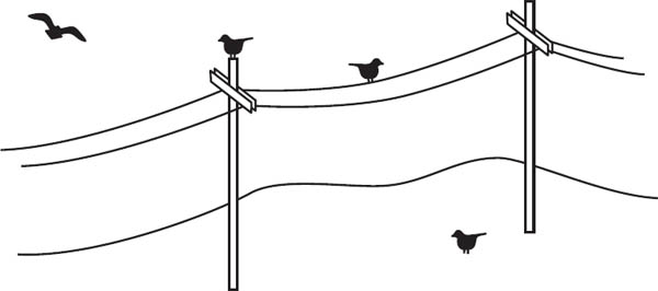
Figure 22.1. Birds experiencing dimensions 0, 1, 2, and 3.
It is common to associate dimension with geometric figures such as points, lines, and planes. However, as we saw in the previous chapters, we want a looser definition of dimension than these rigid geometric ones. A more healthy way to think about dimension is in terms of degrees of freedom—the dimension is the number of independent directions that an object can move.
Consider the flock of birds shown in figure 22.1. Each bird has limitations upon where it can move—they each have a different number of degrees of freedom. The bird on the top of the telephone pole cannot move anywhere. It is experiencing zero-dimensional space. The bird on the wire can move side-to-side. It has one degree of freedom, so it inhabits a 1-dimensional space. The bird on the ground is living in 2-dimensional space, and the flying bird is in 3-dimensional space. Notice that we did not speak of straight lines and flat planes, just degrees of freedom. The hanging wire is certainly not straight and the ground has hills and valleys.
Because we live in a 3-dimensional world, it is easy for us to conceptualize dimensions 0, 1, 2, and 3. Four or more dimensions lie outside our realm of experience. When we investigated cross caps, the Klein bottle, and the projective plane, we recognized the need for a fourth dimension. Although it is not easy to imagine this hop into the fourth dimension, it is not too difficult to visualize these surfaces. After all, these 4-dimensional surfaces are mostly 3-dimensional. Topological entities that require more than a brief detour into the fourth dimension are another story.
It is common to hear people say that time is the fourth dimension. This perspective is due to Joseph-Louis Lagrange and has been around since 1788.1 Time is a quantity with which we are familiar, and it may help get a handle on 4-dimensional space. But there is a downside. We cannot ignore the “arrow of time.” The three physical dimensions that we encounter have no direction. Particles can move back and forth on a line without contradicting the laws of physics. However, that same particle cannot go backward and forward in time. There is something inherently different about time compared to the other three dimensions. In general we do not want our fourth dimension to have this restrictive property.
In practice, high-dimensional spaces arise naturally. Predicting the motion of the space shuttle requires six dimensions—three dimensions for its position and three dimensions for its velocity. To pinpoint the positions and velocities of the sun, earth, and moon, we need eighteen. An economist’s financial model, an ecologist’s population study, and a physicist’s quantum theory may each possess a large number of variables (each of which contributes a dimension). From a mathematical point of view we can add as many dimensions as we need.
Regardless of the source of our high-dimensional space, in our discussion we assume that each dimension is physical, that each is no different from the three usual dimensions. We are not asserting that there are more than three physical dimensions. Perhaps there are, and perhaps there are not (physicists studying string theory claim that there are at least ten dimensions). Mathematically speaking, this is irrelevant.
We denote n-dimensional Euclidean space by ![]() n.
n. ![]() 1 is the set of real numbers—the number line that we study in grade school. Each point can be represented by a single x-value.
1 is the set of real numbers—the number line that we study in grade school. Each point can be represented by a single x-value. ![]() 2 is the infinite plane. It has an x- and a y-axis, and using these coordinate axes, each point can be represented by an ordered pair (x, y). Three-dimensional Euclidean space is denoted
2 is the infinite plane. It has an x- and a y-axis, and using these coordinate axes, each point can be represented by an ordered pair (x, y). Three-dimensional Euclidean space is denoted ![]() 3 and each point in
3 and each point in ![]() 3 is uniquely represented by an ordered triple (x, y, z). Mathematically, it is trivial to extend these notions to n-dimensional Euclidean space. Each point in
3 is uniquely represented by an ordered triple (x, y, z). Mathematically, it is trivial to extend these notions to n-dimensional Euclidean space. Each point in ![]() n can be uniquely described by an ordered n-tuple, (x1, x2, . . . , xn). We can work with these high-dimensional spaces whether they exist physically or not.
n can be uniquely described by an ordered n-tuple, (x1, x2, . . . , xn). We can work with these high-dimensional spaces whether they exist physically or not.
We spent a lot of time learning about surfaces. We described surfaces as being locally two dimensional. An ant living on the surface has two degrees of freedom. We can extend this same idea to higher-dimensional shapes. An n-dimensional manifold, or n-manifold, is a topological object that looks locally like n-dimensional Euclidean space. An inhabitant of one of these manifolds has n degrees of freedom. Just as was the case with surfaces, manifolds exhibit local simplicity and global complexity. They may have holes or other nontrivial topology. Regardless of the global characteristics, up close, all n-manifolds look like ![]() n.
n.
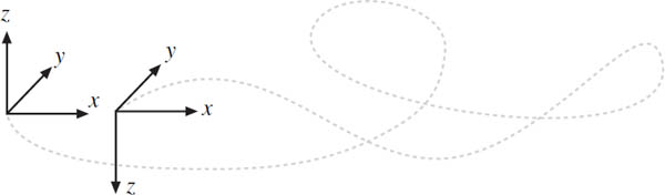
Figure 22.2. Coordinate axes in a nonorientable 3-manifold.
Also like surfaces, n-manifolds can be orientable or nonorientable. The easiest way to test for nonorientability in a manifold is by using Dyck’s criteria (chapter 16). Suppose we had two identical coordinate frames in a nonorientable n-manifold. Then it is possible to move one coordinate frame around the manifold in such a way that when it returns to the first one, it is impossible to get all of the axes to line up correctly. For example, in a nonorientable 3-manifold, when the x- and y-axes are in alignment, the z-axes point in opposite directions (see figure 22.2).
Manifolds of any dimension can have boundaries, and the boundary of an n-manifold is a manifold of one dimension less. The boundary of a 1-manifold is 0-manifold (two points), the boundary of a 2-manifold (a surface) is a 1-manifold (one or more circles), and the boundary of a 3-manifold (a solid) is a surface. For example, the boundary of a solid torus is the usual (hollow) torus. The boundary of a solid ball is a sphere, and more generally, the n-ball, Bn, is an n-manifold and its boundary is the (n − 1)-sphere, Sn−1 (see chapter 19 for the definitions of Sn and Bn).
The history of manifolds dates back to Riemann and his study of multivalued complex functions and the associated Riemann surfaces. But it was near the turn of the twentieth century that Poincaré argued that the manifold was an important object of study, and he gave several ways of describing it. Probably the simplest way is by expressing it as a subset of ![]() n using an equation or equations. For example, x2 + y2 + z2 = 1 is a sphere and
n using an equation or equations. For example, x2 + y2 + z2 = 1 is a sphere and ![]() is a torus. They both reside in
is a torus. They both reside in ![]() 3
3
Sometimes Poincaré presented a manifold as an n-dimensional polyhedron called a simplicial complex. In a simplicial complex, the generalization of a vertex, an edge, and a face is a simplex. We may assume that all of the simplices are triangles, or the higher-dimensional analogue of a triangle. As we see in figure 22.3, a k-simplex is the k-dimensional figure determined by k + 1 points. A 0-simplex is a point, a 1-simplex is a line segment, a 2-simplex is a triangle, a 3-simplex is a triangular pyramid, and so on. In a simplicial complex we assume that when two neighboring simplices meet, they meet along some lower-dimensional simplex. (Note that just as Hessel’s polyhedra [chapter 15] were not surfaces, not every simplicial complex is a manifold.)

Figure 22.3. 0-, 1-, 2-, and 3-simplices.

Figure 22.4. Glue the corresponding faces to obtain a 3-torus.
Yet another way Poincaré described manifolds was by generalizing Klein’s construction of surfaces. Just as Klein created surfaces by gluing together sides of polygons, so did Poincaré create n-manifolds by gluing together the faces of n-dimensional polyhedra. We obtain a torus by gluing opposite sides of a square together without any twists. Likewise, we construct a 3-torus (the 3-dimensional analogue of a torus) by gluing opposite sides of a cube together in pairs with no twists (see figure 22.4). A 3-torus is an example of a closed, orientable 3-manifold.
The abstract definition of manifold does not specify where the manifold “lives.” We were able to define and understand the properties of the Klein bottle without ever knowing that it cannot exist in ![]() 3. We ask, given a generic n-manifold, can we always place it in some Euclidean space,
3. We ask, given a generic n-manifold, can we always place it in some Euclidean space, ![]() m, so that it has no self-intersections? If so, how big does m have to be? Hassler Whitney proved that any n-manifold can be placed in some Euclidean space with dimension at most 2n. This has become known as the Whitney embedding theorem.
m, so that it has no self-intersections? If so, how big does m have to be? Hassler Whitney proved that any n-manifold can be placed in some Euclidean space with dimension at most 2n. This has become known as the Whitney embedding theorem.
In chapter 17 we encountered the classification theorem for surfaces. Every surface is either a sphere with handles or a sphere with cross caps. It is reasonable to ask whether it is possible to classify n-manifolds for n greater than two. It turns out that this is an extremely challenging problem. In chapter 17 we asserted that the dimension of an n-manifold is a topological invariant—that it is impossible for a 5-manifold and a 7-manifold to be homeomorphic. Even this was a difficult result to justify. It was not until 1911 that Brouwer proved the invariance of dimension theorem,2 which states that ![]() n is not homeomorphic to
n is not homeomorphic to ![]() m when m ≠ n. Later we will discuss one of the most famous classification questions, one whose correct solution is worth $1 million.
m when m ≠ n. Later we will discuss one of the most famous classification questions, one whose correct solution is worth $1 million.
The importance of the classification problem should not be understated. One of the basic open questions is, what is the shape of the universe? String theorists aside, it appears that we live in a 3-dimensional universe—a gigantic 3-manifold (presumably without boundary!). What are the properties of this manifold? Is its diameter finite or does it extend forever? Is it topologically the same as ![]() 3 or does it have some nontrivial topological features. Even more bizarre, could it be nonorientable? Is it possible for a right-handed astronaut to fly away from earth, and return left-handed?
3 or does it have some nontrivial topological features. Even more bizarre, could it be nonorientable? Is it possible for a right-handed astronaut to fly away from earth, and return left-handed?
Now that we have the notion of manifolds of all dimensions, it is natural to ask whether we can apply Euler’s formula to them. To do so, we should return to polyhedra. Cauchy was the first to catch a glimpse of the higher- dimensional generalization of Euler’s formula.3 In the same paper in which he proved Euler’s formula by transporting a polyhedron onto a plane, he stated and proved a higher-dimensional analogue of Euler’s formula. He argued that if vertices, edges, and faces are inserted into the interior of a convex polyhedron, dividing it into S convex polyhedra, and if the total number of vertices, edges, and faces (including those in the interior) is V, E, and F, respectively, then
V − E + F − S = 1.
To illustrate Cauchy’s theorem, look at the decompositions of the octahedron and the cube in figure 22.5. A new face in the interior of the octahedron divides it into two polyhedra, so S = 2. There are 6 vertices, 12 edges, and 9 faces. As Cauchy asserted, 6 − 12 + 9 − 2 = 1. Likewise, the cube is divided into 3 polyhedra with 12 vertices, 22 edges, and 14 faces, and 12 − 22 + 14 − 3 = 1.

Figure 22.5. Decompositions of an octahedron and a cube.
In 1852 Ludwig Schläfli discovered a version of Euler’s formula that held for convex polyhedra of all dimensions, but his work was not published in full until 1901 and by then his results had been rediscovered by others.4 Suppose that P is an n-dimensional polyhedron that has b0 vertices, b1 edges, b2 faces, and in general bk facets of dimension k. Schläfli thought of these n-dimensional polyhedra as hollow shells bounded by (n − 1)-dimensional faces; in this case that means bn = 0. Define the Euler number by extending the alternating sum to facets of higher dimension: χ(P) = b0 − b1 + b2 − . . . ± bn−1. Schläfli observed that X(P) = 0 when n is odd and X(P) = 2 when n is even.
Let us examine Cauchy and Schläfli’s results from a modern topological viewpoint. First of all, both Cauchy and Schläfli were considering convex polyhedra, so they did not have holes or tunnels. Topologically, Schläfli’s hollow n-dimensional polyhedron is homeomorphic to the (n − 1)-dimensional sphere, Sn−1. Thus, Schläfli’s theorem shows that X(Sn) = 0 when n is odd and X(Sn) = 2 when n is even. On the other hand, Cauchy assumed his convex polyhedron was solid, so it is topologically the same as the 3-ball, B3. Cauchy proved that χ(B3) = 1, and we now know that X(Bn) = 1 for all n. To see this, create Bn by “filling in” Schläfli’s polyhedron with one n-dimensional facet. So χ(Bn) = X(Sn −1) + (−1)n. For n even, χ(Bn) = 0 + 1 = 1; and for n odd, χ(Bn)= 2 − 1 = 1.
The next higher-dimensional generalization was given by Listing. We have met Listing several times already. He contributed to graph theory (chapter 11), he was the first mathematician to study knots (chapter 18), and he discovered the Möbius band before Möbius and even coined the term topology (chapter 16). In fact, he was the first to have a truly topological view of Euler’s formula and was one of the first mathematicians to think like a topologist. One might expect him to be regarded as one of the giants of topology. In reality, he was largely ignored in his lifetime and remained an obscure figure for years after he died. Even now, the Dictionary of Scientific Biography, an eighteen-volume set containing short biographies of the most important scientists and mathematicians in history, contains no entry for Listing.
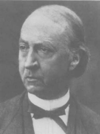
Figure 22.6. Johann Listing.
It is not clear why he never gained his rightful place in history. His academic pedigree was excellent. He was a doctoral student of Gauss, and he remained in his mentor’s inner circle until the day Gauss died (Listing was actually present at his death). For eight years he lived next door to Riemann. (Surprisingly, there is no evidence of collaboration or meaningful conversation between these two who could have shared so much. It has been suggested that Listing may have feared that the tuberculosis that had ravaged Riemann’s family was contagious.5) Listing made important contributions in areas of science as well, such as the optics of the eye. He coined several terms other than topology that have persisted to this day, such as “micron,” the unit for one millionth of a meter.
Perhaps his obscurity was due to his personal attributes. Although he was a gregarious and kind individual, he suffered from manic depression, he was perpetually in financial danger due to his extensive debts, and his wife was often in trouble with the law. Maybe it was his restless spirit that took him away from mathematics for years at a time, his bad career decisions, or his refusal to play the political games in academia. It might have been his way of presenting mathematics. His writing was always too focused on details, making it difficult to perceive the important and deep mathematics that he discovered.

Figure 22.7. A decomposition of a solid torus.
He wrote two monographs on topology, one in 1847 and one in 1861.6 The first, the previously mentioned Topologie, consisted mostly of his topological musings. The second, with the long title of Der Census räumlicher Complexe oder Verallgemeinerung des Euler’schen Satzes von den Polyedern (The Census of Spatial Complexes or Generalization of Euler’s Theorem on Polyhedra), contained his generalizations of Euler’s formula to nonconvex 3-dimensional shapes. In 1884 P. G. Tait lamented that Listing’s writings on topology
have not yet been rescued from their most undeserved obscurity, and published in an English dress, especially when so much that is comparatively worthless, or at least not so worthy, has already secured these honours.7
In Census Listing abandoned the rigid polyhedral view of these shapes; instead he gave the problem a topological treatment. Listing counted the number of vertices, edges, faces, and (3-dimensonal) spaces, but he allowed these features to have nontrivial topology, or cyclosis (as he called it). For instance, he counted a circle as an edge and a sphere as a face, but when he counted them he modified the tally by taking into account their topology. He counted a cylinder as a face, but because it contained a nontrivial loop, he subtracted one. Thus, if A, B, C, and D, are the numbers of vertices, edges, faces, and spaces, each suitably purged of its cyclosis, then A − B + C − D = 0.
To give a flavor of how Listing’s decomposition works, we apply it to the solid torus with the decomposition shown in figure 22.7. It has no vertices, it has a single circular edge, it has two faces (one shaped like a cylinder and one a disk), and it has two spaces (the inside of the cylinder and the ambient space, which he always counted). Because this decomposition has no vertices, A = 0. There is one edge, but it contains a closed loop, so B = 1 − 1 = 0. There are two faces, but since the cylindrical one contains a closed loop around its circumference, C decreases by one. So C = 2 − 1 = 1. Finally, there are two spaces, but since the exterior space contains a nontrivial loop, we have D = 2 − 1 = 1. As predicted by Listing, A − B + C − D = 0 − 0 + 1 − 1 = 0.
Listing’s approach to the problem was remarkably clever and insightful. It was the first attempt to treat the 3-dimensional Euler’s formula in a truly topological way. However, it was far from perfect. At the very least, this means of computing A, B, C, and D was confusing. Listing abandoned all of the beautiful simplicity of Euler’s vertices, edges, and faces. Instead, we must understand the topology of each building block of Listing’s partition.
The next major addition to the theory of n-dimensional topology was made by Riemann and the Italian mathematician Enrico Betti (1823–1892). In order to understand their contributions, we must return to Riemann’s study of surfaces.
In his 1851 doctoral dissertation Riemann presented a topological invariant that counted the number of holes in an orientable surface. He called it the connectivity number of the surface.8 A surface (with or without boundary) has connectivity number n, or is n-connected,* if n is the largest number of cuts that one can make without disconnecting the surface.† If the surface has a boundary, then the cuts must begin and end at the boundary. If the surface has no boundary, then the first cut must begin and end at the same point (thereafter the surface has a boundary).
In figure 22.8 we have three surfaces with boundary: a cylinder, a disk with three holes, and a Möbius band. The dashed lines represent the cuts. The cylinder and the disk with holes have connectivity numbers 1 and 3, respectively. Riemann’s work on connectivity numbers predates Möbius’s discovery of nonorientable surfaces, but we can compute the connectivity numbers for nonorientable surfaces in exactly the same way. So the Möbius band is 1-connected.
The simplest closed surface is the sphere. Any cut along a closed curve will disconnect the sphere. So it is 0-connected. If we cut a torus once around the tube, then it becomes a cylinder. We may then cut it a second time along the length of the cylinder, obtaining a rectangle. The connectivity number of the torus is 2. Similarly, we can compute the connectivity numbers of other surfaces. The double torus is 4-connected, the projective plane is 1-connected, and the Klein bottle is 2-connected.

Figure 22.8. Cuts to determine the connectivity numbers for various surfaces.
Although it may seem that the connectivity number is an important new topological invariant, it is actually the Euler number in disguise. The astute reader may have noticed the relationship between the connectivity number and the genus for orientable closed surfaces. Indeed, Riemann noticed this as well—the connectivity number is simply twice the genus. If we know the genus, the Euler number, or the connectivity number, then we know the other two.
Let us be more precise about the relationship between the connectivity number and the Euler number. Imagine that before we do any cutting, we draw the cut-lines on an n-connected surface, S. This gives a very simple partition of the surface. For the sake of simplicity, we may assume that each cut begins and ends at the same point, so V = 1. At the end of our cutting we have a single face, so F = 1. Moreover, each cut-line is an edge, so E = n. This gives the following simple relationship between the connectivity number and the Euler number:
X(S) = 1 − n + 1 = 2 − n.
Toward the end of his life, Riemann’s health began to decline. Between 1862 and his death in 1866, he made several trips to Italy for convalescence. While he was there, he visited his friend Betti, whom he had met in Göttingen in 1858. Betti was a university professor at the University of Pisa. He had also taught high school, was a member of Parliament, and had served as a senator. He was a renowned mathematician and gifted teacher who was partially responsible for the rebirth of mathematics in Italy after the reunification.
Figure 22.9. Enrico Betti.
During his visits to Italy, Riemann spoke with Betti about how to extend the connectivity numbers to manifolds of higher dimension. It is difficult to say who contributed what to the theory. It was Betti who, in 1871, published these generalizations, but letters and notes show that Riemann knew much of this as early as 1852.
The idea behind the generalizations is that, just as Riemann counted the maximal number of 1-dimensional cuts for a surface, in an n-dimensional manifold we may also count the maximal number of m-dimensional manifolds (subject to somewhat complicated criteria) for each m ≤ n. This gives a connectivity number bm for each m from 0 to n. In this notation, b1 is Riemann’s connectivity number.
Betti proved that these bm were topological invariants for the manifold. However, working with n-manifolds is tricky, and later it became apparent that there were subtle errors with Betti’s arguments and definitions. Nonetheless, Betti’s work was an extremely important step toward understanding the topology of n-manifolds.
It was Henri Poincaré who aimed to fix Betti’s errors. He did that, and much more.
*Today the term n-connected means something slightly different.
†Actually, Riemann’s connectivity number was one larger than this value, but we will keep the smaller value to be consistent with modern notation.