CHAPTER 18
A KNOTTY PROBLEM
One of the earliest topological investigations was the study of knots. We are all familiar with knots. They keep our boats secured to shore, our shoes snug on our feet, and the cables and wires hopelessly tangled behind our computers. These are not, strictly speaking, mathematical knots. A mathematical knot has no free ends; it is a topological circle living in 3-dimensional Euclidean space. (To turn an electrical extension cord into a mathematical knot, simply plug the two ends together.)
In figure 18.1 we see the projections of six mathematical knots: the unknot, trefoil knot, figure eight knot, pentafoil knot, gingerbread man knot (for lack of an accepted name), and square knot.
In the previous chapter we stressed that topologists are usually interested in the intrinsic properties of topological objects, not the extrinsic properties. Knot theory is one notable exception. What is interesting about a knot is how the circle is placed in space—its extrinsic configuration. Intrinsically, they are all identical—every knot is homeomorphic to a circle. So in the study of knots, “the same” does not mean homeomorphic. Instead, two knots are the same if one can be continuously deformed into the other. That is, two knots are the same if there is an isotopy between them. The first three knots in figure 18.2 are isotopic (they are all the same as the unknot) and the last two are the isotopic (they are both the same as the trefoil knot), but as we will see, the unknot is not isotopic to the trefoil knot.
A main goal of knot theory is to classify knots. Just as we did for surfaces, we would like to find tools that allow us to tell whether two knots are the same or different. Ideally, like surfaces, we dream about producing an exhaustive and duplicate-free list of all knots. Right now no such complete list exists, but much has been accomplished in this direction. The meager goal of this chapter is to develop enough tools to prove that the knots in figure 18.1 are all different. One of these tools requires the classification of surfaces and the Euler number.

Figure 18.1. The unknot, trefoil knot, figure eight knot, pentafoil knot, gingerbread man knot, and square knot.

Figure 18.2. Three projections of the unknot and two projections of the trefoil knot.
The study and use of knots is as old as humankind. A vast array of bends, hitches, loops, splices, and nooses have been discovered for every conceivable use. In many cultures knots and their projections were common themes for jewelry and artwork. They were also important in the production of fabrics, for what is a piece of cloth if not a giant knot? In comparison, the mathematical study of knots is considerably younger; the first mathematical investigation dates back to the eighteenth century.
The topological significance of knots was recognized by Alexandre-Théophile Vandermonde (1735–1796) in 1771, only thirty-five years after Euler’s bridges of Königsberg paper. Vandermonde’s short paper “Remarques sur les problèmes de situation” (“Remarks on the problems of position”) began as follows:
Whatever the twists and turns of a system of threads in space, one can always obtain an expression for the calculation of its dimensions, but the expression will be of little use in practice. The craftsman who fashions a braid, a net, or some knots will be concerned, not with questions of measurement, but with those of position; what he sees there is the manner in which the threads are interlaced.2
Despite the promising start, his paper did not focus on knots but on a topological approach to the so-called “knight’s tours” in chess. Yet, he did give a brief description of how certain textile patterns could be described symbolically.
From his drawings and notes, we know that Gauss thought about knots as early as 1794, but alas, he never published anything on the subject. In one handwritten gem from 1833 he gave a double integral that could be used to compute the linking number of two closed curves—a topological quantity that measures how many times the curves wind around each other.3
Perhaps it is not surprising, then, that Listing, one of Gauss’s students, truly began the mathematical study of knots. His contributions can be found in his 1847 monograph Topologie,4 the oft-cited treasure trove of topological curiosities. Although Listing did not propose the classification of all knots, he was clearly interested in finding techniques for differentiating two knots. For instance, he stated that the trefoil knot and its mirror image are not the same knot. Just as Listing’s treatment of the Möbius band was ignored, so was his study of knots. Ultimately, the rise of knot theory was due not to Listing, but to two Scottish physicists working on a new atomic theory.
In 1867 William Thomson (1824–1907) asserted that atoms were formed by vortices, or knots, in the ether. Perhaps better known as Lord Kelvin, Thomson is also responsible for the absolute temperature scale and for helping design the first transatlantic telegraph cable (he was knighted for this work). According to Kelvin each atom corresponded to a different knot or a linked collection of knots, and that the stability of an atom was due to the stability of the knot under topological deformation. This ingenious but misguided belief prevailed for two decades.
Thomson’s atomic theory led his friend Peter Guthrie Tait to commence the classification of knots. In 1877 Tait began a tabulation of all knots—in his eyes he was creating a periodic table of elements. Eventually this view of chemistry was abandoned, but Tait continued his study. By 1900 he and the Indian-born American mathematician Charles Newton Little (1858–1923) had given an almost complete account of knots with ten or fewer crossings (by crossings, we mean in a given planar drawing—we will say more about this terminology shortly).
Tait primarily used his remarkable intuition to classify knots. In the years afterward, mathematicians devised a myriad of ingenious tools for rigorously differentiating knots. Most of these tools are knot invariants. In chapter 17 we discussed topological invariants for surfaces. Knot invariants play the same role for knots. A knot invariant is a number, or other entity, that is associated to a knot. If the invariants of two knots are different, then they must be different knots.

Figure 18.3. William Thomson (Lord Kelvin) and Peter Guthrie Tait.
There are many knot invariants, and some are quite easy to describe. In this chapter we will introduce a few knot invariants, including one that is related to surfaces and the Euler number.
A knot is a circle, and circles can be found on the boundaries of surfaces. Surprisingly, it is possible to find surfaces with knotted boundaries. In figure 18.4 we see that the unknot is the boundary of a disk (no surprise here) and the trefoil knot is the boundary of a Möbius band with three half-twists. We saw another example of a surface with a trefoil knot boundary in figure 17.10.
Remarkably, not only is it possible to find a surface with a knotted boundary, it turns out that every knot can be realized as the boundary of a surface.
As a fun experiment, try making surfaces with knotted boundaries out of soap bubbles. To do so, make a knot out of stiff wire (a coat hanger will suffice for small knots, although it is too stiff and not long enough to make elaborate knots), then dip it into a bubble solution. Poke holes as needed to form a single surface.*

Figure 18.4. The unknot is the boundary of a disk and the trefoil knot is the boundary of a Möbius band with three half-twists.

Figure 18.5. Herbert Seifert.
The trefoil in figure 18.4 is the boundary of a nonorientable surface (remember that in 3-dimensional space, nonorientable and one-sided are synonymous). It is possible to avoid this situation—given any knot, we are able to construct an orientable surface with this knot as its boundary. Such a surface is called a Seifert surface, named for Herbert Seifert (1907–1996). Perhaps as surprising as this theorem is the simplicity of constructing such surfaces. We will now give Seifert’s elegant algorithm, which he discovered in 1934.5
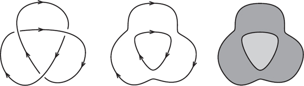
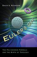
Figure 18.6. Seifert circles for a trefoil knot and the corresponding disks.
We illustrate the algorithm for a trefoil knot. To begin, pick one of the two possible orientations for the knot. That is, pick a direction of travel along the knot. Next, project the knot onto the plane. Almost any projection is allowable. We want to avoid “bad” projections such as those having three strands crossing at the same point or having two sections of string project on top of each other for more than a point, but otherwise the projection can be as complicated as we want.
Next, use this projection to create a collection of circles called Seifert circles. Start tracing the knot following the orientation of the knot. At each crossing, change to the other strand, but still follow the direction of orientation. A circle is obtained when the tracing returns to the starting point (see figure 18.6). Repeat on all untraced strands of the knot. Given these Seifert circles, create disks having these circles as boundaries. Depending on the projection, some of the circles may be nested inside each other. In this case the disks will sit atop one another (as is the case with the trefoil in figure 18.6).
Now, join the disks together by attaching rectangular bands, each with a half-twist. Specifically, at each location where there had been a crossing, attach a twisted band with the direction of the twist determined by the original crossing (see figure 18.7). Although it is not immediately obvious, it is not too difficult to prove that this procedure always produces an orientable surface with boundary.
We complete the construction of the Seifert surface for the trefoil knot in figure 18.8. In figure 18.9 we repeat the process for the square knot. This surface is obtained from three disks and six bands.
According to the powerful classification theorem for surfaces, we “know” every possible surface. A Seifert surface is an orientable surface with one boundary component. Therefore, it must be homeomorphic to a sphere or g-holed torus with a disk removed. Now we truly see the power of the classification theorem, for Seifert surfaces do not look like punctured tori. Theoretically, we could glue a disk onto the boundary of one of these Seifert surfaces and obtain a closed surface, but this gluing would require four dimensions.

Figure 18.7. Attaching a band with a twist.

Figure 18.8. A Seifert surface for a trefoil knot.

Figure 18.9. A Seifert surface for a square knot.
Because we know that a Seifert surface is orientable and has one boundary, we need only know its Euler number to classify it. Suppose S is a Seifert surface constructed from d disks and b bands. Since the Euler number of a disk is 1 (and thus the Euler number of d disjoint disks is d), it suffices to determine the effect of adding a band to a surface.
Suppose we attach both ends of a band to a surface with boundary (that may not be connected). In doing so we add one face, two edges and no vertices to the surface. According to the familiar alternating sum of the Euler number, adding the band decreases the Euler number by 1. So, adding b bands decreases it by b.
A Seifert surface S constructed from d disks and b bands has Euler number χ(S) = d − b.
We constructed the Seifert surface for the trefoil knot (figure 18.8) using two disks and three bands. So its Euler number is −1. Similarly, the Seifert surface for the square knot is made from three disks and six bands, so its Euler number is −3.
If we were to glue a disk to the boundary of a Seifert surface, we would obtain a closed surface of genus g. Doing so adds a face, so this closed surface would have an Euler number one larger than that of the Seifert surface. The Seifert surface for the trefoil knot shown in figure 18.8 has Euler number −1. If we attach a disk to the boundary, then the resulting surface has Euler number 0. It must be a torus—a surface of genus 1. We say that the Seifert surface has genus 1.
We can apply this same logic to any Seifert surface made from d disks and b bands. By attaching a disk to the boundary, we obtain a closed, orientable surface S with Euler number χ(S) = d − b + 1. S is a surface of genus g, and χ(S) = 2 − 2g = d − b + 1. Solving for g we find the genus.
A Seifert surface made from d disks and b bands has genus g = (1 − d + b)/2.
The Seifert surface for the square knot has genus g = (1 − 3 + 6)/2 = 2. It is a 2-holed torus with a disk removed. In figure 18.10 we see Seifert surfaces for the pentafoil, figure eight, and gingerbread man knots. The Seifert surface for the pentafoil knot is constructed from two disks and five bands. So, its genus is (1 − 2 + 5)/2 = 2. The Seifert surface for the figure eight knot is made from three disks and four bands, and has genus (1 − 3 + 4)/2 = 1. The Seifert surface for the gingerbread man knot, made from three disks and six bands, has genus (1 − 3 + 6)/2 = 2.

Figure 18.10. Seifert surfaces for the pentafoil, figure eight, and gingerbread man knots.
It would be nice if the genus of a Seifert surface was a knot invariant. The problem is that a given knot may have more than one topologically distinct Seifert surface (all it would take is to choose a different projection of the knot at the beginning of the process). However, we do not have to abandon this idea entirely. We may define the genus of knot to be the smallest genus of all possible Seifert surfaces. We denote the genus of a knot K by g(K).
The unknot bounds a disk, which is a sphere with a disk removed, so it has genus 0. It is the only knot that bounds a disk, so the genus is a positive number for every knot that is not the unknot.
This definition is somewhat frustrating. While the genus is a perfectly valid knot invariant, in practice it is not easy to compute. We constructed a Seifert surface for the gingerbread man knot and found its genus to be 2. Is that the genus of the knot? Maybe, maybe not. Perhaps it is possible to find a different Seifert surface for this knot with genus 1. It is not clear how to prove that no such Seifert surface exists.
The good news is that we can easily compute the genus for a broad class of knots called alternating knots. Trace the projection of the figure eight knot in figure 18.1 with your finger and observe the behavior at the crossings. The string goes over, under, over, under, over, under, over, and under—it alternates throughout the projection. This projection is called alternating. The projections of the trefoil, pentafoil, and gingerbread man knots are also alternating, but the projection of the square knot is not. A knot is called alternating if it has some alternating projection. The given projection of the square knot is not alternating, but this does not mean that it is not an alternating knot, for it may have another projection that is alternating.

Figure 18.11. An 8-crossing knot that is not alternating.
All of the simplest knots are alternating. Every knot with seven or fewer crossings is alternating, and only three of the 8-crossing knots are not alternating (one is shown in figure 18.11). However, as the number of crossings increases, the relative number of alternating knots drops. Of the 2,404 prime knots (we will define prime shortly) with 12 or fewer crossings, 63% are alternating. Of the roughly 1.7 million prime knots with 16 or fewer crossings, only 29% are alternating.6
What saves us is a theorem proved at the end of the 1950s by Richard H. Crowell and Kunio Murasugi.7
The Seifert surface obtained from an alternating projection is guaranteed to have the minimum genus.
In other words, because the trefoil, figure eight, pentafoil, and gingerbread man knots are alternating, we can say with certainty that their genuses are 1, 1, 2, and 2, respectively. So, none of the four knots is the unknot, and the trefoil and figure eight knots are different from the pentafoil and gingerbread man knots. At this point the reader should be able to prove that the two knots in the introduction (figure I.5) are different.
We now take a brief diversion to determine the genus of the square knot. Prime numbers are the basic building blocks of the positive integers. A number p > 1 is prime if whenever p is the product of two positive integers m and n, either m = 1 or n = 1; otherwise it is composite. In a similar manner we define prime knots, the basic building blocks for all knots. In order to do so we need a way to “multiply” knots.
Given knots K and L, the product of K and L, denoted K#L, is formed as follows. Place the projections of K and L next to (but not overlapping) one another. Cut an outside strand of both knots and join the four ends together without introducing any new crossings. In figure 18.12 we see that the square knot is the product of a trefoil knot and its mirror image (the product of two identical trefoil knots is a granny knot).
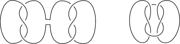
Figure 18.12. The product of a trefoil knot and its mirror image is a square knot.
A knot M is prime if whenever M = K#L, either K or L is the unknot.† In other words, a knot is prime if it cannot be written as the product of two nontrivial knots. A nontrivial knot that is not prime is called composite. Clearly, primality is a knot invariant. We have shown that the square knot is a composite knot. We will not prove it, but the trefoil, figure eight, pentafoil, and gingerbread man knots are all prime, so none of them are isotopic to the square knot.
Suppose we know the genuses of the knots K and L. Is it easy to determine the genus of K#L? Suppose SK and SL are Seifert surfaces for K and L of minimal genus. Using the same projections of K and L, form K#L and its corresponding Seifert surface SK#L. It is not difficult to see that if SK is formed from dK disks and bK bands and SL is formed from dL disks and bL bands, then SK#L is formed from dK + dL − 1 disks and bK + bL bands. So, the genus of SK#L is
The problem is, we do not know if SK#L has the minimal genus for the knot K#L. So all we can conclude is that g(K#L) ≤ g(K) + g(L). We omit the proof, but in fact SK#L does have the minimal genus. Thus, the genus is additive.
For any knots K and L, g(K#L) = g(K) + g(L).
This formula enables us to compute the genus of the square knot:
g(square knot) = g(trefoil knot) + g(trefoil knot) = 1 + 1 = 2.
An interesting consequence of this formula is that if either K or L is not the unknot, then K#L is not the unknot. This follows because if either g(K) ≠ 0 or g(L) ≠ 0, then g(K#L) ≠ 0. Here is a concrete way of understanding this: if your shoelaces are knotted, then it is impossible to take the two free ends of the laces and tie a knot that unties the knot in your laces. Knots do not have “inverse knots” that untie them.
It is worth remarking that if K and L are alternating knots, then K#L is an alternating knot (can you see why this is true?). So the square knot, which we have shown without an alternating projection, has an alternating projection.
While the genus of a knot enables us to differentiate many knots, it is not a complete invariant—just because two knots have the same genus does not mean that they are the same knot. For example, the genuses of the trefoil knot and the figure eight knot are the same. So either these two knots are the same (which they are not), or we need to find a different method to distinguish them. Likewise, the genuses of the pentafoil, the gingerbread man, and the square knot are the same.
In the remainder of this chapter we introduce two more knot invariants that enable us to differentiate the remaining knots. They are just a small sampling of the many known knot invariants.
The first of these invariants is called colorability. To test for colorability, we draw the projection of a knot using three crayons of different colors. The knot is colorable if at each crossing only one color appears or if all three colors appear. Moreover, we insist that the entire projection not be just one color. It is not too difficult to prove that colorability is a knot invariant, but we will skip the proof. In particular, colorability does not depend on the choice of the projection.
In figure 18.13 we see that the trefoil is colorable (we used black, grey, and “dashed” as our three colors). However, a little experimentation shows that the figure eight is not colorable. In the example shown in figure 18.13 we obeyed the rules and colored the first three strands. At this point we run into trouble with the top strand. Each crossing would force this strand to be a different color. There is no color that we can use to color this knot correctly. So the trefoil and the figure eight knots are distinct.
We leave it to the reader to show that the square knot is colorable, but the pentafoil and the gingerbread man knots are not. Thus, we have further proof that the square knot is distinct from the pentafoil and gingerbread man knots.

Figure 18.13. The trefoil is colorable and the figure eight is not.
TABLE 18.1:
The number of prime knots with a given crossing number.

Using primality, genus, and colorability, we are able to differentiate all of our knots except the pentafoil and the gingerbread man knots. Both knots are prime, have genus 2, and are not colorable. To prove that they are distinct we must introduce one more knot invariant: the crossing number.
The crossing number of a knot is the fewest number of crossings of all projections of the knot. We will write c(K) for the crossing number of a knot K. The usual projection of the unknot has no crossings, so it has crossing number O. We know that the trefoil knot and the unknot are different, and we have a projection of the trefoil with 3 crossings. Any knot with zero, one, or two crossings is the unknot, so the crossing number of the trefoil is 3.
Knots are often grouped together by crossing number. There is not a lot of diversity among knots of few crossings. As we see in table 18.1, the trefoil is the only knot with crossing number 3 (not double-counting a knot and its mirror image), and there are only seven prime knots with six or fewer crossings. As the crossing number increases, the variety of knots increases rapidly.8
Like the genus, and for exactly the same reason, the crossing number is often difficult to work with. Given a projection, it is easy to count the number of crossings. However, we cannot guarantee that there is no other projection with fewer crossings. If we have a projection of a knot K with n crossings, all we can say is that c(K) ≤ n. Fortunately, just like the genus, the crossing number is easy to compute for alternating knots.

Figure 18.14. A nonessential crossing.
A century ago Tait conjectured that a reduced alternating projection of a knot exhibits the minimum number of crossings. Here “reduced” means that before counting the number of crossings, we remove all nonessential crossings, such as the crossing in figure 18.14. Such a crossing can be removed by simply giving part of the knot a half-twist. Once these are removed, Tait conjectured, the number of crossings is the minimum. Tait’s conjecture remained open for many years, but was proved independently and almost simultaneously by Louis Kauffman, Kunio Murasugi, and Morwen Thistlethwaite in the mid-1980s.9
A reduced alternating projection of a knot exhibits the minimum number of crossings.
This theorem enables us to compute the crossing number of any alternating knot with ease. Because our projections of the trefoil, figure eight, pentafoil, and gingerbread man knots are already reduced and alternating, it is trivial to determine their crossing numbers. They are 3, 4, 5, and 6, respectively. So with this single invariant we conclude that all of these knots are distinct—including the pentafoil and the gingerbread man knots.
It is worth asking how crossing numbers are related to products of knots. Is there a nice relationship between c(K), c(L), and c(K#L)? If K and L are both alternating, then K#L is alternating. Moreover, by being careful we can take reduced alternating projections of K and L and join them so that the resulting projection of K#L is also reduced and alternating (that is not what we did for the square knot). Consequently, in this special case the crossing number is additive.
If K and L are alternating knots, then c(K#L) = c(K) + c(L).
For instance, c(square knot) = c(trefoil) + c(trefoil) = 3 + 3 = 6.
TABLE 18.2:
A summary of the properties of our knots.
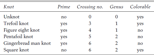
Figure 18.15. Are the gingerbread man and 63 knots the same?
Is the crossing number additive for all knots, just like the genus is? It is an old conjecture that this equality holds for all knots. Surprisingly, no one has discovered a proof, nor an example showing that it is false!
In this chapter we introduced a few of the many important knot invariants, and using them we were able to distinguish the six knots at the beginning of the chapter. We summarize our findings in table 18.2.
With these tools we can make a dent in the classification process. However, they only get us so far. The two projections in figure 18.15—the gingerbread man knot and the so-called 63 knot—are different knots, but our invariants cannot tell them apart. They are both prime, 6-crossing, alternating, not colorable, genus 2 knots. We need more tools to distinguish them.
Also, we have not presented any techniques for showing that two projections are the same knot. We devoted this chapter to showing that two projections are different knots. We encourage the reader to peruse the literature to investigate this interesting area of knot theory.
Mathematicians and scientists have a dysfunctional give-and-take relationship. Naively one would think that they work hand-in-hand. Scientists give problems to the mathematicians to solve and the mathematicians create theories that they hope will be useful to scientists.
The needs of scientists often do spur the creation of new mathematics, just as Kelvin’s vortex model of atomic theory inspired knot theory. But mathematicians do not relish being servants of science. Even when a mathematical theory is born from a practical application, it quickly takes on a life of its own and is advanced for its own inherent properties. Theoretical mathematicians are a stubborn bunch who as a whole are more interested in beauty, truth, elegance, and grandeur than in applicability.
When Kelvin’s atomic model was proved wrong, scientists lost interest in knots, but mathematicians continued studying them. Knot theory took on a life of its own as an area of pure mathematics. For most of the twentieth century it was of interest only to mathematicians. Knot theory remained an active research area with applications to other areas of pure mathematics, but not to science.
But even the most abstract and theoretical areas of mathematics can prove useful. Applicable mathematics often comes from decidedly non-applicable areas. The usefulness of a particular theory is often not clear for many years. No one could have predicted that the study of prime numbers would later enable us to encrypt credit-card information so that it can be sent safely across the Internet. Nineteenth-century mathematicians did not know that their work in non-Euclidean geometry would provide the foundation for Einstein’s theory of general relativity.
Toward the end of the twentieth century the usefulness of knot theory reemerged in the natural sciences. Physicists, biologists, and chemists discovered that the mathematical theory of knots gave them insight into their fields. Whether it is the study of DNA or other large molecules, magnetic field lines, quantum field theory, or statistical mechanics, knot theory now plays an important role.
Mathematicians work in a store that makes and sells tools. Occasionally they take special orders from their scientific customers, but most of the day they toil away making elegant tools, the uses for which have not yet been invented. Scientists visit this tool shop and browse the shelves in hopes that one of the tools fits their needs. The knot-theory aisle of the store, long ignored by scientists, is now bustling with activity. In the next chapter we will see how the emerging ideas of topology and the Euler number created yet another unexpectedly useful tool for scientists.
* To make durable bubbles that can span large distances, we recommend mixing 1 gallon of water, 2/3 cup of dish soap, and 1 tablespoon of glycerin (which can be found at any drugstore). For best results, let the solution sit for a while before use.
† The unknot satisfies this definition of primality, but just as 1 is not considered a prime number, the unknot is not considered a prime knot.